Algoritmul cuantic de optimizare aproximativă

Estimare de utilizare: 22 de minute pe un procesor Heron r3 (NOTĂ: Aceasta este doar o estimare. Durata ta de execuție poate varia.)

Rezultate de învățare

După parcurgerea acestui tutorial, te poți aștepta să înțelegi următoarele informații:

• Cum să mapezi o problemă clasică de optimizare combinatorie (max-cut) la un Hamiltonian cuantic
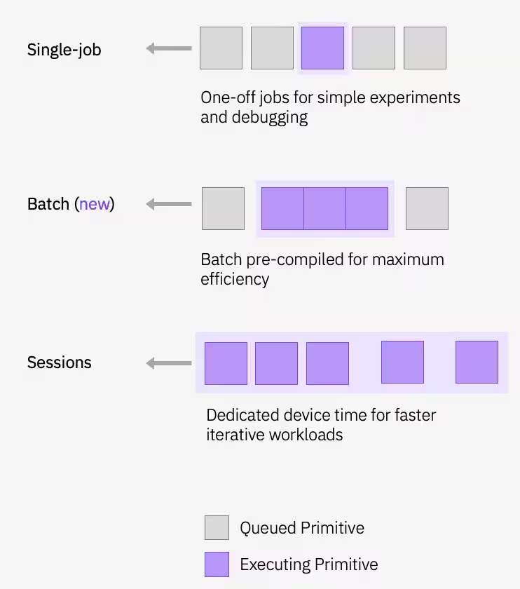
• Cum să implementezi și să rulezi Algoritmul cuantic de optimizare aproximativă (QAOA) folosind sesiuni Qiskit Runtime
• Cum să scalezi un flux de lucru QAOA de la un exemplu mic pe simulator la execuția la scară de utilitate pe hardware

Cerințe preliminare

Este recomandat să te familiarizezi cu aceste subiecte:

• Bazele circuitelor cuantice
• Algoritmi variaționali
• QAOA în profunzime — pentru o tratare cuprinzătoare a algoritmului QAOA și aplicarea lui la scară de utilitate

Context

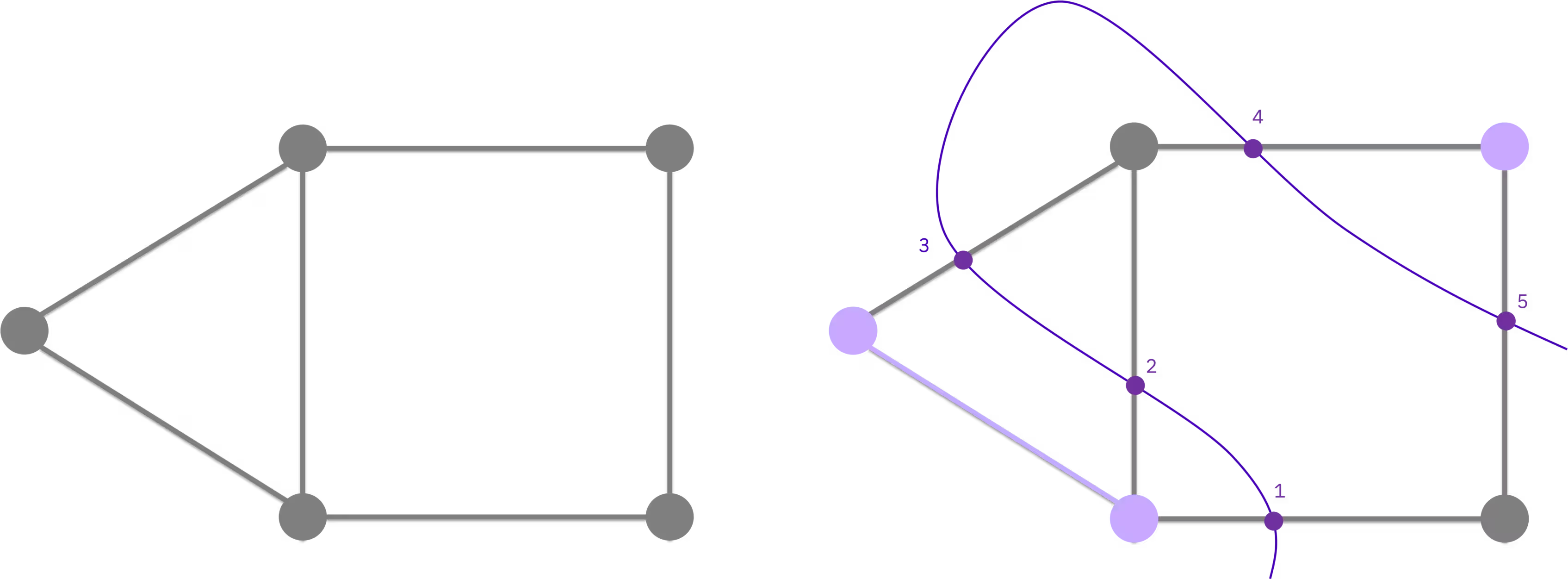
Algoritmul cuantic de optimizare aproximativă (QAOA) este o metodă iterativă hibridă cuantică-clasică pentru rezolvarea problemelor de optimizare combinatorie. În acest tutorial, vei folosi QAOA pentru a rezolva problema tăieturii maxime (max-cut) — o problemă de optimizare NP-hard cu aplicații în clustering, știința rețelelor și fizica statistică. Având un graf de noduri conectate prin muchii, scopul este să împarți nodurile în două mulțimi astfel încât numărul de muchii care traversează partiția să fie maximizat.

De la optimizarea clasică la circuitele cuantice

Max-cut poate fi exprimată ca o problemă clasică de optimizare binară. Fiecărui nod îi este atribuită o variabilă binară $x_i \in \{0, 1\}$ care indică din ce mulțime face parte. Obiectivul este de a maximiza numărul de muchii ale căror capete se află în mulțimi diferite:

$$\max_{x \in \{0,1\}^n} \sum_{(i,j)} x_i + x_j - 2x_ix_j.$$

Aceasta este, în mod echivalent, o problemă de Optimizare Binară Pătratică Fără Constrângeri (QUBO) de forma $\min_x\, x^T Q x$. Printr-o substituție standard de variabile ($x_i \to (1 - Z_i)/2$), problema QUBO poate fi rescrisă ca un Hamiltonian de cost a cărui stare fundamentală codifică soluția optimă. În general, acest Hamiltonian are atât termeni pătratici, cât și termeni liniari:

$$H_C = \sum_{ij} Q_{ij} \, Z_i Z_j + \sum_i b_i \, Z_i.$$

Pentru problema max-cut neponderată considerată aici, coeficienții liniari dispar ($b_i = 0$) și $Q_{ij} = 1$ pentru fiecare muchie, lăsând forma mai simplă $H_C = \sum_{(i,j) \in E} Z_i Z_j$ pe care o vei construi în codul de mai jos. Forma mai generală de mai sus este cea de care ai avea nevoie pentru a adapta acest flux de lucru la grafuri ponderate sau la alte probleme exprimabile prin QUBO.

Cum funcționează QAOA

QAOA pregătește soluții candidate prin aplicarea de straturi alternante a doi operatori unei stări inițiale de suprapunere $H^{\otimes n}|0\rangle$: operatorul de cost $e^{-i\gamma_k H_C}$ și un operator de amestecare (mixer) $e^{-i\beta_k H_m}$. Unghiurile $\gamma_k$ și $\beta_k$ sunt optimizate într-o buclă clasică de feedback; calculatorul cuantic evaluează funcția de cost, iar un optimizator clasic actualizează parametrii până la convergență. Această buclă iterativă rulează în cadrul unei sesiuni Qiskit Runtime, care menține dispozitivul cuantic rezervat pe parcursul iterațiilor pentru o latență mai mică.

Pentru o tratare mai aprofundată a teoriei QAOA, inclusiv derivarea completă de la QUBO la Hamiltonian, vezi modulul de curs QAOA.

În acest tutorial vei rezolva mai întâi max-cut pe un graf mic cu cinci noduri, apoi vei scala același flux de lucru la o problemă la scară de utilitate cu 100 de noduri pe hardware real. Notă privind accesul la plan: Acest tutorial folosește sesiuni Qiskit Runtime, care sunt disponibile doar pe planul Premium. Dacă ești pe planul Open, nu poți rula acest tutorial așa cum este scris; în schimb, va trebui să înlocuiești Session cu modul job (adică să trimiți fiecare iterație ca un job independent, în loc să încadrezi bucla de optimizare într-un with Session(...)). Fluxul de lucru tot rulează, dar fiecare iterație suportă latența completă a cozii, în loc să reutilizeze un dispozitiv rezervat. Vezi Prezentarea generală a planurilor disponibile pentru mai multe informații.

Cerințe

Înainte de a începe acest tutorial, asigură-te că ai instalate următoarele:

• Qiskit SDK v2.0 sau mai recent, cu suport pentru vizualizare
• Qiskit Runtime v0.22 sau mai recent (pip install qiskit-ibm-runtime)

În plus, vei avea nevoie de acces la o instanță pe IBM Quantum® Platform.

Configurare

# Added by doQumentation — required packages for this notebook
!pip install -q matplotlib numpy qiskit qiskit-ibm-runtime rustworkx scipy

import matplotlib.pyplot as plt
import rustworkx as rx
from rustworkx.visualization import mpl_draw as draw_graph
import numpy as np
from scipy.optimize import minimize
from collections import defaultdict
from typing import Sequence

from qiskit.quantum_info import SparsePauliOp
from qiskit.circuit.library import QAOAAnsatz
from qiskit.transpiler.preset_passmanagers import generate_preset_pass_manager

from qiskit_ibm_runtime import QiskitRuntimeService
from qiskit_ibm_runtime import Session, EstimatorV2 as Estimator
from qiskit_ibm_runtime import SamplerV2 as Sampler

Exemplu la scară mică

Această secțiune parcurge fiecare pas al fluxului de lucru QAOA pe o instanță mică de max-cut cu cinci noduri. În ciuda etichetei „scară mică”, acest exemplu rulează totuși pe hardware IBM Quantum real — codul selectează un Backend cu 127 sau mai mulți qubiți și execută circuitul acolo. Inițializează problema ta creând un graf cu $n=5$ noduri.

n_small = 5

graph = rx.PyGraph()
graph.add_nodes_from(np.arange(0, n_small, 1))
edge_list = [
    (0, 1, 1.0),
    (0, 2, 1.0),
    (0, 4, 1.0),
    (1, 2, 1.0),
    (2, 3, 1.0),
    (3, 4, 1.0),
]
graph.add_edges_from(edge_list)
draw_graph(graph, node_size=600, with_labels=True)

Pasul 1: Maparea intrărilor clasice la o problemă cuantică

Mapează graful clasic în circuite și operatori cuantici. După cum este descris în secțiunea Context, pentru max-cut neponderată Hamiltonianul de cost se reduce la $H_C = \sum_{(i,j) \in E} Z_i Z_j$, iar QAOA folosește un circuit ansatz parametrizat pentru a pregăti stări fundamentale candidate ale lui $H_C$.

Construirea Hamiltonianului de cost

Convertește muchiile grafului în termeni Pauli $Z_iZ_j$ pentru a construi $H_C$ (vezi Context pentru derivare).

def build_max_cut_paulis(
    graph: rx.PyGraph,
) -> list[tuple[str, list[int], float]]:
    """Convert graph edges to a list of ZZ Pauli terms.

    The returned list is in the sparse format expected by
    ``SparsePauliOp.from_sparse_list``: each element is
    ``(pauli_string, qubit_indices, coefficient)``.
    """
    pauli_list = []
    for edge in list(graph.edge_list()):
        weight = graph.get_edge_data(edge[0], edge[1])
        pauli_list.append(("ZZ", [edge[0], edge[1]], weight))
    return pauli_list

max_cut_paulis = build_max_cut_paulis(graph)
cost_hamiltonian = SparsePauliOp.from_sparse_list(max_cut_paulis, n_small)
print("Cost Function Hamiltonian:", cost_hamiltonian)

Cost Function Hamiltonian: SparsePauliOp(['IIIZZ', 'IIZIZ', 'ZIIIZ', 'IIZZI', 'IZZII', 'ZZIII'],
              coeffs=[1.+0.j, 1.+0.j, 1.+0.j, 1.+0.j, 1.+0.j, 1.+0.j])

Construirea circuitului ansatz QAOA

Folosește QAOAAnsatz pentru a construi circuitul QAOA parametrizat din Hamiltonianul de cost. Aici folosim reps=2 (două straturi QAOA, patru parametri: $\beta_0, \beta_1, \gamma_0, \gamma_1$).

circuit = QAOAAnsatz(cost_operator=cost_hamiltonian, reps=2)
circuit.measure_all()

circuit.draw("mpl")

circuit.parameters

ParameterView([ParameterVectorElement(β[0]), ParameterVectorElement(β[1]), ParameterVectorElement(γ[0]), ParameterVectorElement(γ[1])])

Pasul 2: Optimizarea problemei pentru execuția pe hardware cuantic

Transpilează circuitul abstract în instrucțiuni native ale hardware-ului. Acest pas gestionează maparea qubiților, descompunerea porților, rutarea și suprimarea erorilor. Vezi documentația despre transpilare pentru mai multe informații.

service = QiskitRuntimeService()
backend = service.least_busy(
    operational=True, simulator=False, min_num_qubits=127
)
print(backend)

# Create pass manager for transpilation. Level 3 is the most aggressive
# preset: slower to transpile, but produces shorter circuits that are
# more robust to hardware noise.
pm = generate_preset_pass_manager(optimization_level=3, backend=backend)

candidate_circuit = pm.run(circuit)
candidate_circuit.draw("mpl", fold=False, idle_wires=False)

<IBMBackend('ibm_pittsburgh')>

Pasul 3: Execuție folosind primitivele Qiskit

Bucla de optimizare QAOA rulează în interiorul unei sesiuni Qiskit Runtime pentru a menține dispozitivul rezervat pe parcursul iterațiilor. Un Estimator evaluează $\langle H_C \rangle$ la fiecare pas, iar un optimizator clasic (COBYLA) actualizează parametrii până la convergență.

Definește parametrii inițiali și rulează bucla de optimizare:

# QAOA doesn't prescribe principled default angles — any bounded choice
# works as a warm start for problems this small. beta and gamma are
# periodic (beta in [0, pi] and gamma in [0, 2*pi] modulo the underlying
# Pauli-rotation periods), and pi/2 and pi are just midpoints of those
# ranges. For harder problems you would typically warm start from known
# good angles or transfer parameters from smaller instances.
initial_gamma = np.pi
initial_beta = np.pi / 2
init_params = [initial_beta, initial_beta, initial_gamma, initial_gamma]

def cost_func_estimator(params, ansatz, hamiltonian, estimator):
    # transform the observable defined on virtual qubits to
    # an observable defined on all physical qubits
    isa_hamiltonian = hamiltonian.apply_layout(ansatz.layout)

    pub = (ansatz, isa_hamiltonian, params)
    job = estimator.run([pub])

    results = job.result()[0]
    cost = results.data.evs

    objective_func_vals.append(cost)

    return cost

objective_func_vals = []  # Global variable
with Session(backend=backend) as session:
    # If using qiskit-ibm-runtime<0.24.0, change `mode=` to `session=`
    estimator = Estimator(mode=session)
    estimator.options.default_shots = 1000

    # Set simple error suppression/mitigation options
    estimator.options.dynamical_decoupling.enable = True
    estimator.options.dynamical_decoupling.sequence_type = "XY4"
    estimator.options.twirling.enable_gates = True
    estimator.options.twirling.num_randomizations = "auto"
    estimator.options.environment.job_tags = ["TUT_QAOA"]

    result = minimize(
        cost_func_estimator,
        init_params,
        args=(candidate_circuit, cost_hamiltonian, estimator),
        method="COBYLA",
        tol=1e-2,
    )
    print(result)

message: Return from COBYLA because the trust region radius reaches its lower bound.
 success: True
  status: 0
     fun: -2.0402211719947774
       x: [ 3.041e+00  1.212e+00  2.081e+00  4.471e+00]
    nfev: 36
   maxcv: 0.0

Optimizatorul a reușit să reducă costul și să găsească parametri mai buni pentru circuit.

O curbă care scade lin și apoi atinge un platou este semnătura convergenței. O curbă zgomotoasă, nemonotonă, indică de obicei că ceva din amonte necesită atenție; cauzele frecvente sunt prea puține shot-uri per evaluare (varianță mare a estimatorului), parametri inițiali slabi sau un circuit a cărui adâncime este dominată de zgomotul hardware-ului. COBYLA este fără derivate și destul de robust la zgomot moderat, dar atunci când zgomotul copleșește îmbunătățirile reale ale costului per pas, modelul său de aproximare liniară nu mai poate distinge descreșterea reală de fluctuațiile aleatorii, iar optimizatorul rătăcește.

plt.figure(figsize=(12, 6))
plt.plot(objective_func_vals)
plt.xlabel("Iteration")
plt.ylabel("Cost")
plt.show()

Atribuie parametrii optimizați și eșantionează distribuția finală folosind primitiva Sampler.

optimized_circuit = candidate_circuit.assign_parameters(result.x)
optimized_circuit.draw("mpl", fold=False, idle_wires=False)

# If using qiskit-ibm-runtime<0.24.0, change `mode=` to `backend=`
sampler = Sampler(mode=backend)
sampler.options.default_shots = 10000

# Set simple error suppression/mitigation options
sampler.options.dynamical_decoupling.enable = True
sampler.options.dynamical_decoupling.sequence_type = "XY4"
sampler.options.twirling.enable_gates = True
sampler.options.twirling.num_randomizations = "auto"

sampler.options.environment.job_tags = ["TUT_QAOA"]

pub = (optimized_circuit,)
job = sampler.run([pub], shots=int(1e4))
counts_int = job.result()[0].data.meas.get_int_counts()
counts_bin = job.result()[0].data.meas.get_counts()
shots = sum(counts_int.values())
final_distribution_int = {key: val / shots for key, val in counts_int.items()}
final_distribution_bin = {key: val / shots for key, val in counts_bin.items()}
print(final_distribution_int)

{18: 0.039, 5: 0.0665, 20: 0.0973, 29: 0.0063, 9: 0.0899, 13: 0.0379, 2: 0.0047, 1: 0.0153, 11: 0.0932, 14: 0.0327, 12: 0.0314, 25: 0.0193, 21: 0.0398, 6: 0.0224, 4: 0.0197, 10: 0.0387, 3: 0.0181, 26: 0.07, 17: 0.0327, 19: 0.0332, 22: 0.0914, 24: 0.007, 0: 0.0033, 8: 0.0066, 30: 0.0158, 28: 0.0169, 27: 0.0222, 16: 0.0073, 7: 0.0057, 23: 0.0062, 15: 0.0054, 31: 0.0041}

Pasul 4: Post-procesarea și returnarea rezultatului în formatul clasic dorit

Extrage cel mai probabil șir de biți din distribuția eșantionată. Acesta reprezintă cea mai bună tăietură găsită de QAOA.

# auxiliary functions to sample most likely bitstring
def to_bitstring(integer, num_bits):
    result = np.binary_repr(integer, width=num_bits)
    return [int(digit) for digit in result]

keys = list(final_distribution_int.keys())
values = list(final_distribution_int.values())
most_likely = keys[np.argmax(np.abs(values))]
most_likely_bitstring = to_bitstring(most_likely, len(graph))
most_likely_bitstring.reverse()

print("Result bitstring:", most_likely_bitstring)

Result bitstring: [0, 0, 1, 0, 1]

plt.rcParams.update({"font.size": 10})
final_bits = final_distribution_bin
values = np.abs(list(final_bits.values()))
top_4_values = sorted(values, reverse=True)[:4]
positions = []
for value in top_4_values:
    positions.append(np.where(values == value)[0])
fig = plt.figure(figsize=(11, 6))
ax = fig.add_subplot(1, 1, 1)
plt.xticks(rotation=45)
plt.title("Result Distribution")
plt.xlabel("Bitstrings (reversed)")
plt.ylabel("Probability")
ax.bar(list(final_bits.keys()), list(final_bits.values()), color="tab:grey")
for p in positions:
    ax.get_children()[int(p[0])].set_color("tab:purple")
plt.show()

Vizualizarea celei mai bune tăieturi

Din șirul de biți optim, poți apoi vizualiza această tăietură pe graful original.

# auxiliary function to plot graphs
def plot_result(G, x):
    colors = ["tab:grey" if i == 0 else "tab:purple" for i in x]
    pos, _default_axes = rx.spring_layout(G), plt.axes(frameon=True)
    rx.visualization.mpl_draw(
        G, node_color=colors, node_size=100, alpha=0.8, pos=pos
    )

plot_result(graph, most_likely_bitstring)

Acum, calculează valoarea tăieturii:

def evaluate_sample(x: Sequence[int], graph: rx.PyGraph) -> float:
    assert len(x) == len(
        list(graph.nodes())
    ), "The length of x must coincide with the number of nodes in the graph."
    return sum(
        x[u] * (1 - x[v]) + x[v] * (1 - x[u])
        for u, v in list(graph.edge_list())
    )

cut_value = evaluate_sample(most_likely_bitstring, graph)
print("The value of the cut is:", cut_value)

The value of the cut is: 5

Pentru un graf atât de mic, optimul real este ușor de obținut prin forță brută, așa că poți verifica rezultatele comparând rezultatul QAOA cu răspunsul exact.

# Classical baseline: enumerate all 2**n_small bitstrings and take the best cut.
def brute_force_max_cut(graph: rx.PyGraph) -> tuple[int, list[int]]:
    n = len(list(graph.nodes()))
    best_cut = -1
    best_x: list[int] = []
    for i in range(2**n):
        x = [(i >> k) & 1 for k in range(n)]
        cut = evaluate_sample(x, graph)
        if cut > best_cut:
            best_cut = int(cut)
            best_x = x
    return best_cut, best_x

classical_best, classical_x = brute_force_max_cut(graph)
print(f"Classical optimum (brute force): {classical_best}")
print(f"QAOA cut value:                  {cut_value}")

Classical optimum (brute force): 5
QAOA cut value:                  5

Exemplu pe hardware la scară mare

Ai acces la multe dispozitive cu peste 100 de qubiți pe IBM Quantum Platform. Selectează unul pe care să rezolvi max-cut pe un graf ponderat cu 100 de noduri. Aceasta este o problemă la „scară de utilitate”. Fluxul de lucru urmează aceiași pași ca mai sus, aplicați unui graf mult mai mare.

Flux de lucru cap-coadă la scară de utilitate

Toți cei patru pași sunt prezentați mai jos, aplicați grafului cu 100 de noduri. Structura este aceeași ca în parcursul la scară mică: mapează, transpilează, execută, post-procesează — dar cu o problemă mai mare și împărțită pe cele patru celule de mai jos pentru claritate.

# Precomputed parity lookup table: _PARITY[b] = +1 if popcount(b) is even, else -1.
# We use this to vectorize expectation-value evaluation across all Pauli terms.
_PARITY = np.array(
    [-1 if bin(i).count("1") % 2 else 1 for i in range(256)],
    dtype=np.complex128,
)

def evaluate_sparse_pauli(state: int, observable: SparsePauliOp) -> complex:
    """Expectation value of a SparsePauliOp on a single computational-basis state.

    For a Z-only observable (which QAOA cost Hamiltonians are, after the
    QUBO-to-Hamiltonian mapping), the eigenvalue of each Pauli term on a
    computational-basis state is simply (-1)**popcount(z_mask AND state),
    i.e., the parity of the bitwise-AND of the term's Z-support and the
    measured bitstring.

    This routine packs the Z-support of every Pauli term into bytes, ANDs
    them against the measured state in a single vectorized op, and looks up
    the parity in _PARITY. For a 100-qubit / ~hundreds-of-terms Hamiltonian
    over 10_000 samples, this is dramatically faster than calling
    SparsePauliOp.expectation_value per sample.
    """
    packed_uint8 = np.packbits(observable.paulis.z, axis=1, bitorder="little")
    state_bytes = np.frombuffer(
        state.to_bytes(packed_uint8.shape[1], "little"), dtype=np.uint8
    )
    reduced = np.bitwise_xor.reduce(packed_uint8 & state_bytes, axis=1)
    return np.sum(observable.coeffs * _PARITY[reduced])

def best_solution(samples, hamiltonian):
    """Return the sampled bitstring (as int) with the lowest Hamiltonian cost."""
    min_cost = float("inf")
    min_sol = None
    for bit_str in samples.keys():
        candidate_sol = int(bit_str)
        fval = evaluate_sparse_pauli(candidate_sol, hamiltonian).real
        if fval <= min_cost:
            min_cost = fval
            min_sol = candidate_sol
    return min_sol

def _plot_cdf(objective_values: dict, ax, color):
    x_vals = sorted(objective_values.keys(), reverse=True)
    y_vals = np.cumsum([objective_values[x] for x in x_vals])
    ax.plot(x_vals, y_vals, color=color)

def plot_cdf(dist, ax, title):
    _plot_cdf(dist, ax, "C1")
    ax.vlines(min(list(dist.keys())), 0, 1, "C1", linestyle="--")
    ax.set_title(title)
    ax.set_xlabel("Objective function value")
    ax.set_ylabel("Cumulative distribution function")
    ax.grid(alpha=0.3)

def samples_to_objective_values(samples, hamiltonian):
    """Convert the samples to values of the objective function."""
    objective_values = defaultdict(float)
    for bit_str, prob in samples.items():
        candidate_sol = int(bit_str)
        fval = evaluate_sparse_pauli(candidate_sol, hamiltonian).real
        objective_values[fval] += prob
    return objective_values

Pasul 1: Construiește graful, Hamiltonianul de cost și ansatz-ul.

# Step 1: build the 100-node graph, cost Hamiltonian, and QAOA ansatz.
n_large = 100
graph_100 = rx.PyGraph()
graph_100.add_nodes_from(np.arange(0, n_large, 1))
elist = []
for edge in backend.coupling_map:
    if edge[0] < n_large and edge[1] < n_large:
        elist.append((edge[0], edge[1], 1.0))
graph_100.add_edges_from(elist)

max_cut_paulis_100 = build_max_cut_paulis(graph_100)
cost_hamiltonian_100 = SparsePauliOp.from_sparse_list(
    max_cut_paulis_100, n_large
)

circuit_100 = QAOAAnsatz(cost_operator=cost_hamiltonian_100, reps=1)
circuit_100.measure_all()

Pasul 2: Transpilează pentru Backend-ul hardware selectat.

# Step 2: transpile for hardware.
pm = generate_preset_pass_manager(optimization_level=3, backend=backend)
candidate_circuit_100 = pm.run(circuit_100)

Pasul 3: Rulează bucla de optimizare QAOA în interiorul unei sesiuni, apoi eșantionează.

# Step 3: run the QAOA optimization loop on the device, then sample the
# final distribution with the optimized parameters.
initial_gamma = np.pi
initial_beta = np.pi / 2
init_params = [initial_beta, initial_gamma]

objective_func_vals = []  # Global variable
with Session(backend=backend) as session:
    estimator = Estimator(mode=session)
    estimator.options.default_shots = 1000

    # Set simple error suppression/mitigation options
    estimator.options.dynamical_decoupling.enable = True
    estimator.options.dynamical_decoupling.sequence_type = "XY4"
    estimator.options.twirling.enable_gates = True
    estimator.options.twirling.num_randomizations = "auto"
    estimator.options.environment.job_tags = ["TUT_QAOA"]

    result = minimize(
        cost_func_estimator,
        init_params,
        args=(candidate_circuit_100, cost_hamiltonian_100, estimator),
        method="COBYLA",
    )
    print(result)

# Assign optimal parameters and sample the final distribution.
optimized_circuit_100 = candidate_circuit_100.assign_parameters(result.x)

sampler = Sampler(mode=backend)
sampler.options.default_shots = 10000

# Set simple error suppression/mitigation options
sampler.options.dynamical_decoupling.enable = True
sampler.options.dynamical_decoupling.sequence_type = "XY4"
sampler.options.twirling.enable_gates = True
sampler.options.twirling.num_randomizations = "auto"

# Add a unique tag to the job execution
sampler.options.environment.job_tags = ["TUT_QAOA"]

pub = (optimized_circuit_100,)
job = sampler.run([pub], shots=int(1e4))

counts_int = job.result()[0].data.meas.get_int_counts()
shots = sum(counts_int.values())
final_distribution_100_int = {
    key: val / shots for key, val in counts_int.items()
}

message: Return from COBYLA because the trust region radius reaches its lower bound.
 success: True
  status: 0
     fun: -17.172689238986344
       x: [ 2.574e+00  4.166e+00]
    nfev: 28
   maxcv: 0.0

Pasul 4: Post-procesează distribuția eșantionată pentru a extrage cea mai bună tăietură.

# Step 4: find the best-cost sample and evaluate its cut value.
best_sol_100 = best_solution(final_distribution_100_int, cost_hamiltonian_100)
best_sol_bitstring_100 = to_bitstring(int(best_sol_100), len(graph_100))
best_sol_bitstring_100.reverse()

print("Result bitstring:", best_sol_bitstring_100)

cut_value_100 = evaluate_sample(best_sol_bitstring_100, graph_100)
print("The value of the cut is:", cut_value_100)

Result bitstring: [1, 1, 0, 1, 1, 0, 1, 1, 1, 0, 1, 0, 1, 1, 1, 0, 1, 1, 1, 1, 0, 0, 1, 0, 0, 1, 1, 0, 1, 0, 1, 0, 1, 1, 0, 1, 1, 0, 0, 0, 0, 0, 1, 1, 0, 1, 0, 0, 0, 1, 0, 0, 1, 0, 1, 0, 0, 1, 1, 1, 1, 1, 0, 1, 0, 1, 0, 0, 0, 1, 0, 1, 0, 1, 0, 0, 0, 0, 1, 0, 0, 1, 0, 1, 1, 1, 1, 0, 1, 0, 1, 0, 1, 1, 1, 0, 1, 1, 1, 0]
The value of the cut is: 156

Verifică dacă costul minimizat în bucla de optimizare a convers și vizualizează rezultatele.

# Plot convergence
plt.figure(figsize=(12, 6))
plt.plot(objective_func_vals)
plt.xlabel("Iteration")
plt.ylabel("Cost")
plt.show()

# Visualize the cut
plot_result(graph_100, best_sol_bitstring_100)

# Plot cumulative distribution function
result_dist = samples_to_objective_values(
    final_distribution_100_int, cost_hamiltonian_100
)
fig, ax = plt.subplots(1, 1, figsize=(8, 6))
plot_cdf(result_dist, ax, backend.name)

Pașii următori

Dacă ai găsit interesantă această lucrare, te-ar putea interesa următoarele materiale:

Recomandări

• Tehnici avansate pentru QAOA — explorează strategii avansate pentru îmbunătățirea performanței QAOA
• Provocare de optimizare multi-obiectiv — pune-ți abilitățile la încercare cu această provocare comunitară de optimizare cuantică multi-obiectiv
• Documentația despre transpilare pentru reglarea fină a optimizării circuitelor
• Suprimarea și atenuarea erorilor pentru îmbunătățirea rezultatelor pe hardware