Diagonalizarea cuantică Krylov a Hamiltonienilor de rețea

Estimare de utilizare: 70 de minute pe un procesor Heron sau Nighthawk (NOTĂ: Aceasta este doar o estimare. Durata de execuție poate varia.)

Rezultate ale învățării

• Cum să interpretezi diagonalizarea cuantică Krylov (KQD) ca învățarea unei funcții Hamiltoniene finite care acționează ca un filtru spectral.

• Cum să construiești matricile Hamiltonianului proiectat și de suprapunere cu măsurători swap-test extinse.

• Cum să rezolvi problema generalizată de valori proprii (GEVP) rezultată și să recuperezi o estimare a energiei stării fundamentale pentru un Hamiltonian de rețea.

Cerințe preliminare

• Primitivele Qiskit

• Estimarea energiei stării fundamentale a lanțului Heisenberg cu VQE

• Cursul de algoritmi de diagonalizare cuantică

Context

Acest tutorial demonstrează cum să implementezi algoritmul Krylov de diagonalizare cuantică (KQD) în contextul tiparelor Qiskit. Vei învăța mai întâi teoria din spatele algoritmului, apoi vei vedea o demonstrație a execuției sale pe un QPU.

Estimarea proprietăților de energie joasă ale Hamiltonienilor cu mai multe corpuri este o sarcină centrală în simularea cuantică. De exemplu, energiile stării fundamentale și excitațiile de energie joasă sunt legate direct de stabilitatea chimică, ordinea magnetică, tranzițiile de fază cuantice și răspunsul materialelor. Pe un computer clasic, dimensiunea spațiului Hilbert crește exponențial cu numărul de orbitali sau spinuri, astfel încât diagonalizarea directă devine rapid impracticabilă.

Există mai multe abordări de calcul cuantic pentru această problemă. Metodele variaționale pe termen scurt, cum ar fi rezolvatorul variațional cuantic de valori proprii (VQE), utilizează circuite parametrizate relativ puțin adânci, dar necesită o buclă de optimizare clasică neliniară cu multe evaluări de circuite cuantice. La cealaltă extremă, estimarea cuantică a fazei (QPE) oferă o rută mai directă către estimarea valorilor proprii cu garanții riguroase, dar QPE standard necesită circuite coerente lungi și este potrivit în principal pentru computere cuantice tolerante la erori. KQD se situează între aceste două abordări: folosește evoluția Hamiltoniană în timp real, ca în algoritmii bazați pe estimarea fazei, dar înlocuiește estimarea completă a fazei cu o problemă compactă de valori proprii proiectată, care poate fi rezolvată clasic.

Considerăm un Hamiltonian de $n$ qubiți $H$ și o stare de referință $\lvert \psi_{0}\rangle$. Metoda KQD construiește un subspațiu Krylov din stări evoluate în timp real,

$$\begin{equation*} \lvert \psi_\ell\rangle = e^{-i\ell\Delta t H}\lvert \psi_{0}\rangle, \qquad \ell = 0,1,\ldots,r-1, \end{equation*}$$

unde $r$ este dimensiunea Krylov iar $\Delta t$ este pasul de timp. Orice stare din subspațiul Krylov este apoi reprezentată ca o combinație liniară a acestor stări de bază,

$$\begin{equation*} \lvert \psi(\mathbf{c})\rangle = \frac{\sum_{\ell=0}^{r-1} c_\ell \lvert \psi_\ell\rangle} {\left\|\sum_{\ell=0}^{r-1} c_\ell \lvert \psi_\ell\rangle\right\|}, \end{equation*}$$

where the denominator normalizes the state.

Cu algebră simplă, putem vedea că energia corespunzătoare se scrie ca raportul Rayleigh,

$$\begin{equation*} E(\mathbf{c}) =\langle \psi(\mathbf{c})|H|\psi(\mathbf{c}) \rangle= \frac{ \sum_{k,\ell} c_k^* c_\ell \langle \psi_k\vert H\vert\psi_\ell\rangle }{ \sum_{k,\ell} c_k^* c_\ell \langle \psi_k\vert\psi_\ell\rangle } = \frac{ \mathbf{c}^{\dagger}\mathcal{H}\mathbf{c} }{ \mathbf{c}^{\dagger}\mathcal{S}\mathbf{c} }. \end{equation*}$$

Aici, matricele $\mathcal{S}$ și $\mathcal{H}$,

$$\begin{equation*} \mathcal{S}_{k\ell}=\langle \psi_k\vert\psi_\ell\rangle, \qquad \mathcal{H}_{k\ell}=\langle \psi_k\vert H\vert\psi_\ell\rangle \end{equation*}$$

definesc matricele de suprapunere proiectată și cea Hamiltoniană proiectată. Elementele lor sunt estimate folosind măsurători de circuite cuantice.

Ne propunem să găsim coeficientul $\mathbf{c}$ care dă minimul $E(\mathbf{c})$:

$$\begin{equation*} \min_{\mathbf{c}\neq \mathbf{0}} E(\mathbf{c}). \end{equation*}$$

Conform teoremei Rayleigh-Ritz, această minimizare este echivalentă cu rezolvarea problemei generalizate de valori proprii (GEVP),

$$\begin{equation*} \mathcal{H}\mathbf{c}=E \mathcal{S}\mathbf{c}. \end{equation*}$$

Rețineți că dimensiunea $r$ poate fi suficient de mică pentru ca un computer clasic să rezolve GEVP.

Acesta este același principiu variațional folosit în diagonalizarea subspațiilor clasice, dar aici stările de bază sunt generate prin evoluție cuantică în timp. Comparativ cu VQE, KQD necesită de obicei circuite mai adânci deoarece se bazează pe evoluția în timp real. În schimb, KQD evită optimizarea neliniară a parametrilor și execuția iterativă pe hardware cuantic, și se îmbunătățește sistematic pe măsură ce subspațiul proiectat este extins. Algoritmul a fost demonstrat la scară largă pe hardware cuantic existent [2], iar performanța sa poate fi analizată cu garanții demonstrabile [1].

Cerințe

Înainte de a începe acest tutorial, asigură-te că ai instalate următoarele:

• Qiskit SDK v2.3 sau versiune ulterioară cu suport pentru vizualizare

• Qiskit Runtime v0.22 sau versiune ulterioară ( pip install qiskit-ibm-runtime )

• SciPy (pip install scipy)

• Matplotlib (pip install matplotlib)

• Pandas (pip install pandas)

Execuția pe hardware necesită qiskit-ibm-runtime și acces la un cont IBM Quantum®.

Configurare

Celula de configurare importă modulele necesare și definește funcții ajutătoare pentru flux de lucru:

1. construiește Hamiltonianul Heisenberg;

2. rezolvă GEVP-ul prin prag;

3. evaluează filtrul Krylov învățat;

4. convertește valorile filtrului în ponderi spectrale;

5. reprezintă grafic distribuțiile de energie de referință și filtrată.

# Added by doQumentation — required packages for this notebook
!pip install -q matplotlib numpy pandas qiskit qiskit-ibm-runtime scipy

from __future__ import annotations

import warnings

import numpy as np
import pandas as pd
import scipy.linalg as la
import matplotlib.pyplot as plt

from qiskit import QuantumCircuit, transpile
from qiskit.circuit import Parameter
from qiskit.circuit.library import PauliEvolutionGate
from qiskit.primitives import StatevectorEstimator
from qiskit.quantum_info import Operator, SparsePauliOp
from qiskit.synthesis import LieTrotter, SuzukiTrotter
from qiskit.transpiler import PassManager, Layout
from qiskit.transpiler.passes import CommutativeOptimization
from qiskit.transpiler.preset_passmanagers import generate_preset_pass_manager
from qiskit_ibm_runtime import QiskitRuntimeService, EstimatorV2, Batch
from qiskit_ibm_runtime.fake_provider import FakeMarrakesh

warnings.filterwarnings("ignore")

def make_heisenberg_hamiltonian(
    num_qubits: int,
    coupling: float = 1.0,
) -> SparsePauliOp:
    """Make a Heisenberg Hamiltonian for a 1D chain of qubits with nearest-neighbor interactions."""
    terms: list[tuple[str, complex]] = []

    def append_term(q0: int, q1: int, pauli: str):
        label = ["I"] * num_qubits
        label[num_qubits - 1 - q0] = pauli[0]
        label[num_qubits - 1 - q1] = pauli[1]
        terms.append(("".join(label), coupling))

    for pauli in ("XX", "YY", "ZZ"):
        for q in range(num_qubits - 1):
            append_term(q, q + 1, pauli)
    return SparsePauliOp.from_list(terms).simplify()

def _basis_state_transition_amplitude_sparse(
    hamiltonian: SparsePauliOp,
    bra_state: int,
    ket_state: int,
) -> complex:
    """Evaluate <bra_state|H|ket_state> for computational-basis states."""
    num_qubits = hamiltonian.num_qubits
    amplitude = 0.0 + 0.0j
    for pauli, coeff in zip(hamiltonian.paulis, hamiltonian.coeffs):
        new_state = ket_state
        phase = 1.0 + 0.0j
        for q in range(num_qubits):
            x = bool(pauli.x[q])
            z = bool(pauli.z[q])
            if not x and not z:
                continue
            bit = (new_state >> q) & 1
            if x and z:
                # Y|0> = i|1>, Y|1> = -i|0>
                phase *= 1j if bit == 0 else -1j
                new_state ^= 1 << q
            elif x:
                new_state ^= 1 << q
            else:
                # Z|0> = |0>, Z|1> = -|1>
                if bit:
                    phase *= -1
        if new_state == bra_state:
            amplitude += coeff * phase
    return amplitude

def basis_state_expectation_sparse(
    hamiltonian: SparsePauliOp,
    bitstring: str,
) -> complex:
    """Evaluate <bitstring|H|bitstring>."""
    state = int(bitstring, 2)
    return _basis_state_transition_amplitude_sparse(
        hamiltonian,
        bra_state=state,
        ket_state=state,
    )

def diagonalize_single_1_subspace(
    hamiltonian: SparsePauliOp,
) -> np.ndarray:
    """Diagonalize the Hamiltonian projected onto the single-excitation subspace."""
    num_qubits = hamiltonian.num_qubits

    # Integer basis states |...010...>, with the excitation at qubit k.
    basis = [1 << k for k in range(num_qubits)]

    h_single = np.empty((num_qubits, num_qubits), dtype=complex)

    for row, bra_state in enumerate(basis):
        for col, ket_state in enumerate(basis):
            h_single[row, col] = _basis_state_transition_amplitude_sparse(
                hamiltonian,
                bra_state=bra_state,
                ket_state=ket_state,
            )
    # Remove floating-point-level asymmetry.
    h_single = 0.5 * (h_single + h_single.conj().T)
    evals, _ = np.linalg.eigh(h_single)
    return np.real(evals)

def simple_transpilation(circuit: QuantumCircuit) -> QuantumCircuit:
    """Transpilation to simplify the circuit"""
    pm = PassManager(
        [
            CommutativeOptimization(),
        ]
    )
    circuit = transpile(circuit, optimization_level=3)
    circuit = pm.run(circuit)
    return circuit

def summarize_circuit(circuit: QuantumCircuit) -> dict[str, int | str]:
    """Summarize the circuit with depth, size, and 2-qubit gate information."""
    two_qubit_total = sum(
        inst.operation.num_qubits == 2 for inst in circuit.data
    )
    two_qubit_depth = circuit.depth(lambda x: x[0].num_qubits == 2)
    return {
        "depth": circuit.depth(),
        "size": circuit.size(),
        "2q gates": two_qubit_total,
        "2q depth": two_qubit_depth,
    }

def solve_thresholded_gevp(
    h_matrix: np.ndarray,
    s_matrix: np.ndarray,
    threshold: float = 1e-10,
) -> tuple[float, np.ndarray, int]:
    """Solve H c = E S c using canonical orthogonalization of S."""
    s_vals, s_vecs = la.eigh(s_matrix)

    valid = s_vals > threshold
    if not np.any(valid):
        raise ValueError(
            "All overlap eigenvalues were removed by thresholding."
        )

    keep = valid

    orthogonalizer = s_vecs[:, keep] @ np.diag(1.0 / np.sqrt(s_vals[keep]))
    h_orth = orthogonalizer.conj().T @ h_matrix @ orthogonalizer
    h_orth = 0.5 * (h_orth + h_orth.conj().T)

    eigvals, eigvecs = la.eigh(h_orth)

    coeffs = orthogonalizer @ eigvecs[:, 0]
    normalization = np.sqrt(np.real(coeffs.conj().T @ s_matrix @ coeffs))
    coeffs /= normalization

    return float(np.real(eigvals[0])), coeffs, int(np.sum(keep))

În prima parte a acestui tutorial, demonstrăm metoda KQD folosind un simulator local de stare vectorială. Ulterior, folosim un backend cuantic real pentru a aborda o problemă la scară utilitară.

De asemenea, definim un backend fals pentru a demonstra transpilarea specifică backend-ului și pentru a inspecta circuitul rezultat.

try:
    service = QiskitRuntimeService()
except Exception:
    QiskitRuntimeService.save_account(
        token="<api_token>", instance="<instance>", overwrite=True
    )
    service = QiskitRuntimeService()

backend = FakeMarrakesh()

Exemplu de simulator la scară mică

Pasul 1: Maparea intrărilor clasice la o problemă cuantică

Hamiltonianul și starea de referință

Acest exemplu folosește un lanț Heisenberg cu 12 qubiți și margini deschise ($n=12$),

$$\begin{equation*} H=\sum_{i=0}^{n-2}\left(X_iX_{i+1}+Y_iY_{i+1}+Z_iZ_{i+1}\right), \end{equation*}$$

cu o stare produs cu o singură excitație

$$\begin{equation*} |\psi_{0}\rangle=|000001000000\rangle \end{equation*}$$

ca stare de referință. Deoarece Hamiltonianul Heisenberg definit mai sus conservă numărul total de excitații, starea de referință rămâne în subspațiul cu o singură excitație, a cărui dimensiune crește doar liniar cu numărul de qubiți. Prin urmare, putem calcula eficient energia exactă a stării fundamentale, prin diagonalizarea Hamiltonianului restrâns la acel subspațiu, și îl folosim exclusiv ca reper de diagnostic pentru estimarea KQD. Fluxul de lucru KQD în sine estimează elementele matriceale proiectate folosind primitivele Qiskit și rezolvă clasic problema proiectată rezultată.

# Problem definition for the simulator example
num_qubits = 12
hamiltonian = make_heisenberg_hamiltonian(num_qubits=num_qubits, coupling=1.0)
ref_bitstring = "000001000000"
ref_energy = basis_state_expectation_sparse(hamiltonian, ref_bitstring)

print("Hamiltonian:")
print(hamiltonian)
print(f"Reference state: |{ref_bitstring}>")
print("Reference energy: ", ref_energy)

Hamiltonian:
SparsePauliOp(['IIIIIIIIIIXX', 'IIIIIIIIIXXI', 'IIIIIIIIXXII', 'IIIIIIIXXIII', 'IIIIIIXXIIII', 'IIIIIXXIIIII', 'IIIIXXIIIIII', 'IIIXXIIIIIII', 'IIXXIIIIIIII', 'IXXIIIIIIIII', 'XXIIIIIIIIII', 'IIIIIIIIIIYY', 'IIIIIIIIIYYI', 'IIIIIIIIYYII', 'IIIIIIIYYIII', 'IIIIIIYYIIII', 'IIIIIYYIIIII', 'IIIIYYIIIIII', 'IIIYYIIIIIII', 'IIYYIIIIIIII', 'IYYIIIIIIIII', 'YYIIIIIIIIII', 'IIIIIIIIIIZZ', 'IIIIIIIIIZZI', 'IIIIIIIIZZII', 'IIIIIIIZZIII', 'IIIIIIZZIIII', 'IIIIIZZIIIII', 'IIIIZZIIIIII', 'IIIZZIIIIIII', 'IIZZIIIIIIII', 'IZZIIIIIIIII', 'ZZIIIIIIIIII'],
              coeffs=[1.+0.j, 1.+0.j, 1.+0.j, 1.+0.j, 1.+0.j, 1.+0.j, 1.+0.j, 1.+0.j, 1.+0.j,
 1.+0.j, 1.+0.j, 1.+0.j, 1.+0.j, 1.+0.j, 1.+0.j, 1.+0.j, 1.+0.j, 1.+0.j,
 1.+0.j, 1.+0.j, 1.+0.j, 1.+0.j, 1.+0.j, 1.+0.j, 1.+0.j, 1.+0.j, 1.+0.j,
 1.+0.j, 1.+0.j, 1.+0.j, 1.+0.j, 1.+0.j, 1.+0.j])
Reference state: |000001000000>
Reference energy:  (7+0j)

Stabilirea parametrilor algoritmului

Pe baza limitelor superioare ale normei Hamiltoniene, Ref. [1] sugerează euristic pasul de timp $\Delta t$ ca $\pi/\|H\|$. Deoarece norma spectrală $\|H\|$ este greu de calculat, folosim în schimb limita ei superioară:

$$\begin{equation*} \|H\| \le \sum_{i=0}^{n-2}\underbrace{\|X_i X_{i+1}+Y_{i} Y_{i+1}+Z_{i} Z_{i+1}\|}_{4 \times 4 \text{ matrix, easy to calculate the norm}} = 3(n-1). \end{equation*}$$

Setăm dimensiunea Krylov la $r=10$ și numărul de pași Trotter per pas de timp la $5$: un spațiu Krylov suficient de mare pentru a rezolva spectrul de energie joasă, menținând totodată circuitul cel mai adânc ($t_{\max}=(r-1)\Delta t$) accesibil, și suficienți pași Trotter pentru a menține mică eroarea de discretizare la acel circuit cel mai adânc.

dt = np.pi / (3 * (num_qubits - 1))
print("dt in Krylov basis:  ", dt)

krylov_dim = 10
num_trotter_steps = 5

dt in Krylov basis:   0.09519977738150888

Construirea circuitului

Aici, construim circuitele pentru a estima elementele matriceale $\mathcal{H}_{k\ell}$ și $\mathcal{S}_{k\ell}$. Deoarece toate puterile lui $H$ comută, avem

$$\begin{equation*} \mathcal{H}_{k\ell} = \langle\psi_{0}|H e^{-i(\ell-k)\Delta tH}|\psi_{0}\rangle=\mathcal{H}_{0,\ell-k}, \qquad \mathcal{S}_{k\ell} = \langle\psi_{0}|e^{-i(\ell-k)\Delta tH}|\psi_{0}\rangle=\mathcal{S}_{0,\ell-k}. \end{equation*}$$

Such matrices where the elements depend on the index differences in this manner are called Toeplitz and can be reconstructed from first-row elements indexed by $d=\ell-k$.

Aici, prezentăm circuitul, numit extended-swap-test, care pregătește

$$\begin{equation*} |\Phi_{0d}\rangle= \frac{|0\rangle|\psi_0\rangle+|1\rangle|\psi_d\rangle}{\sqrt{2}}, \end{equation*}$$

unde $|\psi_d\rangle=e^{-id\Delta tH}|\psi_{0}\rangle$.

Starea de referință

Pregătim starea de referință $|\psi_0\rangle$.

qc_ref = QuantumCircuit(num_qubits)
for i, b in enumerate(reversed(ref_bitstring)):
    if b == "1":
        qc_ref.x(i)
display(qc_ref.draw("mpl", scale=0.5))

Evoluția temporală

Realizăm operatorul de evoluție temporală generat de Hamiltonian, aproximat prin simpla Lie-Trotterizare.

t = Parameter("t")

evol_gate = PauliEvolutionGate(
    hamiltonian,
    time=t,
    synthesis=LieTrotter(reps=num_trotter_steps),
    label="U(t)",
)

# Synthesize U(t) first and then control the synthesized circuit.
# This makes the controlled structure visible in the circuit drawer.
evolution_circuit = QuantumCircuit(num_qubits, name="U(t)")
evolution_circuit.append(evol_gate, range(num_qubits))
evolution_circuit = simple_transpilation(evolution_circuit)

# Make a controlled version of the evolution circuit.
controlled_evolution_gate = evolution_circuit.to_gate(label="U(t)").control(
    1, label="C-U(t)"
)
display(
    evolution_circuit.assign_parameters({t: 1.5}).draw(
        "mpl", scale=0.5, fold=-1
    )
)

Testul de swap extins [3]

Circuitul pregătește mai întâi starea de referință pe registrul de sistem, în timp ce ancila rămâne în $|0\rangle$:

$$\begin{equation*} |0\rangle |0\rangle^{\otimes n} \longrightarrow |0\rangle |\psi_{0}\rangle . \end{equation*}$$

Apoi, aplicarea unei porți Hadamard asupra ancilei creează o suprapunere coerentă a două ramuri:

$$\begin{equation*} |0\rangle |\psi_0\rangle \longrightarrow \frac{|0\rangle + |1\rangle}{\sqrt{2}} |\psi_0\rangle = \frac{|0\rangle|\psi_0\rangle + |1\rangle|\psi_0\rangle}{\sqrt{2}} . \end{equation*}$$

În final, se aplică poarta controlată de evoluție temporală:

$$\begin{equation*} U(t=d\Delta t) = e^{-id\Delta t H} \end{equation*}$$

doar când ancila se află în ramura $|1\rangle$. Prin urmare,

$$\begin{equation*} \frac{|0\rangle|\psi_0\rangle + |1\rangle|\psi_0\rangle}{\sqrt{2}} \longrightarrow \frac{|0\rangle|\psi_0\rangle + |1\rangle U(d\Delta t)|\psi_0\rangle}{\sqrt{2}} . \end{equation*}$$

În următorul bloc de cod, implementăm:

$$\begin{equation*} |\Psi(t)\rangle = \frac{|0\rangle|\psi_0\rangle + |1\rangle U(t)|\psi_0\rangle}{\sqrt{2}}, \end{equation*}$$

care va fi atribuit ca $t=d\Delta t$ pentru $d=1,\cdots r-1$ în pasul de execuție.

ancilla = 0
system_qubits = list(range(1, num_qubits + 1))

extended_swap_test = QuantumCircuit(num_qubits + 1)

# Append state preparation part
extended_swap_test = extended_swap_test.compose(qc_ref, system_qubits)

# Prepare the coherent branch label, (|0> + |1>) / sqrt(2).
extended_swap_test.h(ancilla)

# Apply U(t) only to the |1> branch of the ancilla.
extended_swap_test.append(
    controlled_evolution_gate, [ancilla] + system_qubits
)

# Decompose once more for visualization so that control bullets are visible.
display(extended_swap_test.draw("mpl", fold=-1))

Observabile

Pentru orice observabilă hermitiană de sistem $O$, stabilim aici observabilele de calculat:

$$\begin{equation*} z=\langle \psi_0|O|\psi_d\rangle . \end{equation*}$$

Aceasta se întâmplă deoarece $O=I$ dă elementul de suprapunere $\mathcal{S}_{0d}=\langle\psi_0|\psi_d\rangle$, în timp ce $O=H$ dă elementul Hamiltonian $\mathcal{H}_{0d}=\langle\psi_0|H|\psi_d\rangle$.

Folosind $X=|0\rangle\langle 1|+|1\rangle\langle 0|$, avem

$$\begin{align*} \langle \Psi_{0d}|X\otimes O| \Psi_{0d} \rangle &= \left(\frac{\langle0|\langle\psi_0| + \langle1| \langle\psi_d|}{\sqrt{2}}\right)(X\otimes O)\left(\frac{|0\rangle|\psi_0\rangle + |1\rangle |\psi_d\rangle}{\sqrt{2}}\right) \\ &= \frac{1}{2} \left( \langle \psi_0|O|\psi_d\rangle + \langle \psi_d|O|\psi_0\rangle \right) \\ &= \frac{z+z^*}{2} = \operatorname{Re} z. \end{align*}$$

În mod similar, folosind $Y=-i|0\rangle\langle 1|+i|1\rangle\langle 0|$,

$$\begin{align*} \langle \Psi_{0d}|Y\otimes O| \Psi_{0d} \rangle &= \left(\frac{\langle0|\langle\psi_0| + \langle1| \langle\psi_d|}{\sqrt{2}}\right)(Y\otimes O)\left(\frac{|0\rangle|\psi_0\rangle + |1\rangle |\psi_d\rangle}{\sqrt{2}}\right) \\ &= \frac{1}{2} \left( -i\langle \psi_0|O|\psi_d\rangle + i\langle \psi_d|O|\psi_0\rangle \right) \\ &= \frac{-iz+iz^*}{2} = \operatorname{Im} z. \end{align*}$$

Prin urmare, avem

$$\begin{equation*} \langle \Phi_{0d}|X\otimes O|\Phi_{0d}\rangle = \operatorname{Re}\langle\psi_0|O|\psi_d\rangle , \quad \langle \Phi_{0d}|Y\otimes O|\Phi_{0d}\rangle = \operatorname{Im}\langle\psi_0|O|\psi_d\rangle . \end{equation*}$$

În final, pentru fiecare stare $|\Psi_{0d}\rangle$, trebuie să măsurăm:

$$\begin{align*} X \otimes I \text{ pentru } \operatorname{Re}\mathcal{S}_{0d},\\ Y \otimes I \text{ pentru } \operatorname{Im}\mathcal{S}_{0d},\\ X \otimes H \text{ pentru } \operatorname{Re}\mathcal{H}_{0d},\\ Y \otimes H \text{ pentru } \operatorname{Im}\mathcal{H}_{0d}.\\ \end{align*}$$

n_qubits = hamiltonian.num_qubits

observable_labels = [
    "Re S_0d",
    "Im S_0d",
    "Re H_0d",
    "Im H_0d",
]

# X ⊗ I and Y ⊗ I.
# Qiskit's Pauli-label convention places qubit 0 on the rightmost character,
# so the ancilla Pauli is appended to the right.
obs_x_identity = SparsePauliOp("I" * n_qubits + "X")
obs_y_identity = SparsePauliOp("I" * n_qubits + "Y")

# X ⊗ H and Y ⊗ H.
obs_x_hamiltonian = SparsePauliOp.from_list(
    [
        (label + "X", coeff)
        for label, coeff in zip(
            hamiltonian.paulis.to_labels(),
            hamiltonian.coeffs,
        )
    ]
)

obs_y_hamiltonian = SparsePauliOp.from_list(
    [
        (label + "Y", coeff)
        for label, coeff in zip(
            hamiltonian.paulis.to_labels(),
            hamiltonian.coeffs,
        )
    ]
)

observables = [
    obs_x_identity,
    obs_y_identity,
    obs_x_hamiltonian,
    obs_y_hamiltonian,
]

for obs, label in zip(observables, observable_labels):
    print(f"Observable: {label}")
    print(obs)
    print()

Observable: Re S_0d
SparsePauliOp(['IIIIIIIIIIIIX'],
              coeffs=[1.+0.j])

Observable: Im S_0d
SparsePauliOp(['IIIIIIIIIIIIY'],
              coeffs=[1.+0.j])

Observable: Re H_0d
SparsePauliOp(['IIIIIIIIIIXXX', 'IIIIIIIIIXXIX', 'IIIIIIIIXXIIX', 'IIIIIIIXXIIIX', 'IIIIIIXXIIIIX', 'IIIIIXXIIIIIX', 'IIIIXXIIIIIIX', 'IIIXXIIIIIIIX', 'IIXXIIIIIIIIX', 'IXXIIIIIIIIIX', 'XXIIIIIIIIIIX', 'IIIIIIIIIIYYX', 'IIIIIIIIIYYIX', 'IIIIIIIIYYIIX', 'IIIIIIIYYIIIX', 'IIIIIIYYIIIIX', 'IIIIIYYIIIIIX', 'IIIIYYIIIIIIX', 'IIIYYIIIIIIIX', 'IIYYIIIIIIIIX', 'IYYIIIIIIIIIX', 'YYIIIIIIIIIIX', 'IIIIIIIIIIZZX', 'IIIIIIIIIZZIX', 'IIIIIIIIZZIIX', 'IIIIIIIZZIIIX', 'IIIIIIZZIIIIX', 'IIIIIZZIIIIIX', 'IIIIZZIIIIIIX', 'IIIZZIIIIIIIX', 'IIZZIIIIIIIIX', 'IZZIIIIIIIIIX', 'ZZIIIIIIIIIIX'],
              coeffs=[1.+0.j, 1.+0.j, 1.+0.j, 1.+0.j, 1.+0.j, 1.+0.j, 1.+0.j, 1.+0.j, 1.+0.j,
 1.+0.j, 1.+0.j, 1.+0.j, 1.+0.j, 1.+0.j, 1.+0.j, 1.+0.j, 1.+0.j, 1.+0.j,
 1.+0.j, 1.+0.j, 1.+0.j, 1.+0.j, 1.+0.j, 1.+0.j, 1.+0.j, 1.+0.j, 1.+0.j,
 1.+0.j, 1.+0.j, 1.+0.j, 1.+0.j, 1.+0.j, 1.+0.j])

Observable: Im H_0d
SparsePauliOp(['IIIIIIIIIIXXY', 'IIIIIIIIIXXIY', 'IIIIIIIIXXIIY', 'IIIIIIIXXIIIY', 'IIIIIIXXIIIIY', 'IIIIIXXIIIIIY', 'IIIIXXIIIIIIY', 'IIIXXIIIIIIIY', 'IIXXIIIIIIIIY', 'IXXIIIIIIIIIY', 'XXIIIIIIIIIIY', 'IIIIIIIIIIYYY', 'IIIIIIIIIYYIY', 'IIIIIIIIYYIIY', 'IIIIIIIYYIIIY', 'IIIIIIYYIIIIY', 'IIIIIYYIIIIIY', 'IIIIYYIIIIIIY', 'IIIYYIIIIIIIY', 'IIYYIIIIIIIIY', 'IYYIIIIIIIIIY', 'YYIIIIIIIIIIY', 'IIIIIIIIIIZZY', 'IIIIIIIIIZZIY', 'IIIIIIIIZZIIY', 'IIIIIIIZZIIIY', 'IIIIIIZZIIIIY', 'IIIIIZZIIIIIY', 'IIIIZZIIIIIIY', 'IIIZZIIIIIIIY', 'IIZZIIIIIIIIY', 'IZZIIIIIIIIIY', 'ZZIIIIIIIIIIY'],
              coeffs=[1.+0.j, 1.+0.j, 1.+0.j, 1.+0.j, 1.+0.j, 1.+0.j, 1.+0.j, 1.+0.j, 1.+0.j,
 1.+0.j, 1.+0.j, 1.+0.j, 1.+0.j, 1.+0.j, 1.+0.j, 1.+0.j, 1.+0.j, 1.+0.j,
 1.+0.j, 1.+0.j, 1.+0.j, 1.+0.j, 1.+0.j, 1.+0.j, 1.+0.j, 1.+0.j, 1.+0.j,
 1.+0.j, 1.+0.j, 1.+0.j, 1.+0.j, 1.+0.j, 1.+0.j])

Pentru estimarea elementelor matriceale $\mathcal{H}$, numărul de termeni Pauli este mult mai mare decât cel pentru elementele matriceale $\mathcal{S}$.

Putem acum reduce numărul de termeni Hamiltonieni măsurați folosind o tehnică de deplasare [4]. Împărțim Hamiltonianul astfel:

$$\begin{equation*} H = (H-T) + T, \end{equation*}$$

unde $T$ este ales astfel încât starea de referință să fie starea sa proprie,

$$\begin{equation*} T|\psi_0\rangle = \tau |\psi_0\rangle . \end{equation*}$$

Then,

$$\begin{align*} \mathcal{H}_{0d} &= \langle\psi_0|H|\psi_d\rangle \\ &= \langle\psi_0|(H-T)|\psi_d\rangle + \langle\psi_0|T|\psi_d\rangle \\ &= \langle\psi_0|(H-T)|\psi_d\rangle + \tau \langle\psi_0|\psi_d\rangle \\ &= \widetilde{\mathcal{H}}_{0d} + \tau \mathcal{S}_{0d}. \end{align*}$$

Here,

$$\begin{equation*} \widetilde{\mathcal{H}}_{0d} = \langle\psi_0|(H-T)|\psi_d\rangle \end{equation*}$$

este elementul matriceal Hamiltonian deplasat. Prin urmare, trebuie doar să măsurăm $X\otimes (H-T)$ și $Y\otimes (H-T)$. Contribuția de la $T$ este reconstruită clasic folosind elementul matriceal de suprapunere deja măsurat $\mathcal{S}_{0d}$.

În acest exemplu, o alegere naturală este partea diagonală a Hamiltonianului Heisenberg,

$$\begin{equation*} T = \sum_{i=0}^{n-2} Z_iZ_{i+1}. \end{equation*}$$

Deoarece starea de referință este o stare de bază computațională, ea este o stare proprie pentru fiecare termen $Z_iZ_{i+1}$.

Totuși, o alegere mai avantajoasă este să includem nu doar termenii diagonali $ZZ$, ci și termenii $XX+YY$ care anulează starea de referință.

Pentru fiecare pereche vecină, operatorul $XX+YY$ satisface

$$\begin{equation*} (XX+YY)|00\rangle = 0, \qquad (XX+YY)|11\rangle = 0, \end{equation*}$$

and

$$\begin{equation*} (XX+YY)|01\rangle = 2|10\rangle, \qquad (XX+YY)|10\rangle = 2|01\rangle . \end{equation*}$$

Prin urmare, termenul $XX+YY$ contribuie doar atunci când cei doi qubiți vecini au ocupări diferite în șirul de biți de referință. Dacă ambii qubiți sunt fie $0$, fie $1$, termenul anulează starea de referință și poate fi de asemenea deplasat în afară.

Fie $|\psi_{\rm ref}\rangle = |z_0\cdots z_{n-1}\rangle$, unde $z_i \in \{0,1\}$. Astfel, putem alege

$$\begin{equation*} T=\sum_{i=0}^{n-2} Z_iZ_{i+1} + \sum_{z_i={z_{i+1}}} \left( X_iX_{i+1} + Y_iY_{i+1} \right). \end{equation*}$$

Acest operator satisface în continuare

$$\begin{equation*} T|\psi_0\rangle = \tau |\psi_0\rangle , \end{equation*}$$

deoarece termenii $ZZ$ acționează diagonal pe $|\psi_0\rangle$, în timp ce termenii deplasați $XX+YY$ dau zero. Valoarea proprie corespunzătoare este așadar determinată doar de termenii $ZZ$,

$$\begin{equation*} \tau = \sum_{i=0}^{n-2} (-1)^{z_i} (-1)^{z_{i+1}} . \end{equation*}$$

Cu această alegere, Hamiltonianul deplasat devine:

$$\begin{equation*} H-T = \sum_{z_i\ne z_{i+1}} \left( X_iX_{i+1} + Y_iY_{i+1} \right). \end{equation*}$$

Ca rezultat, trebuie măsurate doar muchiile cu ocupări diferite în starea de referință. Toți termenii $ZZ$ și toți termenii $XX+YY$ inactivi sunt reconstruiți prin contribuția de suprapunere $\tau \mathcal{S}_{0d}$, sau dau o contribuție zero prin construcție.

Aceasta oferă o observabilă mai mică decât deplasarea doar a părții diagonale. În special, pentru o stare de referință de bază computațională cu o excitație localizată, doar muchiile adiacente excitației rămân în $H-T$. Prin urmare, numărul de termeni Pauli din $X\otimes(H-T)$ și $Y\otimes(H-T)$ poate fi redus substanțial, în timp ce elementul matriceal reconstruit

$$\begin{equation*} \widetilde{\mathcal{H}}_{0d} + \tau \mathcal{S}_{0d} \end{equation*}$$

rămâne exact același.

def make_reduced_heisenberg_observables(
    ref_bitstring: str,
    coupling: float = 1.0,
) -> tuple[SparsePauliOp, SparsePauliOp, float]:
    """Build X⊗(H-T), Y⊗(H-T), and tau."""
    n_qubits = len(ref_bitstring)

    shifted_terms: list[tuple[str, complex]] = []
    tau = 0.0

    def bit(q: int) -> str:
        return ref_bitstring[n_qubits - 1 - q]

    def append_term(q0: int, q1: int, pauli: str):
        label = ["I"] * n_qubits
        label[n_qubits - 1 - q0] = pauli[0]
        label[n_qubits - 1 - q1] = pauli[1]
        shifted_terms.append(("".join(label), coupling))

    for q in range(n_qubits - 1):
        same_occupation = bit(q) == bit(q + 1)

        # ZZ contribution to tau
        tau += coupling * (1.0 if same_occupation else -1.0)

        # XX + YY survives only for opposite occupations.
        if not same_occupation:
            append_term(q, q + 1, "XX")
            append_term(q, q + 1, "YY")

    if shifted_terms:
        obs_x_shifted_hamiltonian = SparsePauliOp.from_list(
            [(label + "X", coeff) for label, coeff in shifted_terms]
        )
        obs_y_shifted_hamiltonian = SparsePauliOp.from_list(
            [(label + "Y", coeff) for label, coeff in shifted_terms]
        )
    else:
        obs_x_shifted_hamiltonian = SparsePauliOp(
            "I" * n_qubits + "X", coeffs=[0.0]
        )
        obs_y_shifted_hamiltonian = SparsePauliOp(
            "I" * n_qubits + "Y", coeffs=[0.0]
        )

    return obs_x_shifted_hamiltonian, obs_y_shifted_hamiltonian, tau

obs_x_shifted_hamiltonian, obs_y_shifted_hamiltonian, shift_tau = (
    make_reduced_heisenberg_observables(ref_bitstring)
)

print("Observable: Re shifted H_0d")
print(obs_x_shifted_hamiltonian)
print()

print("Observable: Im shifted H_0d")
print(obs_y_shifted_hamiltonian)
print()

print("tau =", shift_tau)

observables = [
    obs_x_identity,
    obs_y_identity,
    obs_x_shifted_hamiltonian,
    obs_y_shifted_hamiltonian,
]
observable_labels = [
    "Re S_0d",
    "Im S_0d",
    "Re shifted H_0d",
    "Im shifted H_0d",
]

Observable: Re shifted H_0d
SparsePauliOp(['IIIIIXXIIIIIX', 'IIIIIYYIIIIIX', 'IIIIXXIIIIIIX', 'IIIIYYIIIIIIX'],
              coeffs=[1.+0.j, 1.+0.j, 1.+0.j, 1.+0.j])

Observable: Im shifted H_0d
SparsePauliOp(['IIIIIXXIIIIIY', 'IIIIIYYIIIIIY', 'IIIIXXIIIIIIY', 'IIIIYYIIIIIIY'],
              coeffs=[1.+0.j, 1.+0.j, 1.+0.j, 1.+0.j])

tau = 7.0

Pasul 2: Optimizează problema pentru execuția pe hardware cuantic

Acum transformăm circuitul abstract extended-swap-test într-un șablon orientat pe hardware. Înainte de asta, optimizăm mai întâi circuitul suplimentar la nivel abstract.

Compararea ordinii termenilor Hamiltonieni

Mai întâi, comparăm ordini diferite ale termenilor Pauli din Hamiltonianul Heisenberg pentru simularea Hamiltoniană. Hamiltonianul în sine rămâne neschimbat, dar ordinea afectează modul în care este generat circuitul cu formulă produs și cât de mult poate fi paralelizată structura în circuit. De exemplu, ordinea naivă listează mai întâi toți termenii $XX$ ai celor mai apropiați vecini, apoi toți termenii $YY$, apoi toți termenii $ZZ$. Aceasta plasează muchii adiacente precum $(0,1)$ și $(1,2)$ una lângă alta, deci nu pot fi executate în paralel. Ordinea pară-apoi-impară vizitează mai întâi muchiile pare disjuncte, urmate de cele impare, ceea ce expune straturi paralele cu doi qubiți. Ordinea grupată pe muchii pară-impară merge un pas mai departe: pentru fiecare muchie, păstrează împreună termenii locali $XX$, $YY$ și $ZZ$, vizitând totuși muchiile pare înaintea celor impare. Ne așteptăm ca ordinile pară-apoi-impară și grupată pe muchii pară-impară să reducă adâncimea circuitului expunând straturi paralele cu doi qubiți, iar ordinea grupată pe muchii să reducă suplimentar eroarea Trotter deoarece interacțiunea locală de doi qubiți pe aceeași muchie este tratată ca un bloc compact.

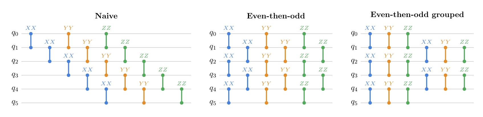
Ordinea Hamiltonianului afectează de asemenea eroarea Trotter. Dacă plasăm termeni care nu comută unul lângă altul, tranzițiile de bază apar mai des, ceea ce induce mai multă eroare Trotter. Grupând termenii care necesită aceeași transformare de bază Pauli, se pot evita schimbările de bază redundante.

Aici, comparația folosește cel mai mare timp de evoluție care apare în estimările Krylov din primul rând, $t_{\max} = (r-1)\Delta t,$ folosind aceeași condiție de transpilare.

Pentru a măsura eroarea Trotter, folosim infidelitatea de proces dintre circuitul Trotterizat și evoluția Hamiltoniană exactă,

$$\begin{equation*} \text{Infidelity}(U,V) = 1-F(U,V) = 1 - \frac{|\operatorname{Tr}(U^\dagger V)|^2}{d^2}, \end{equation*}$$

where $d=2^n$ is the dimension of the Hilbert space.

Acest diagnostic folosește matrici dense, deci este potrivit pentru acest exemplu mic de 12 qubiți, dar nu este conceput ca o subrutină scalabilă.

# The comparison uses the largest time that appears in the first-row Krylov estimates.
# Circuit depth does not depend on this numeric value, but the Trotter error does.
comparison_time = (krylov_dim - 1) * dt

def make_heisenberg_hamiltonian_ordered(
    num_qubits: int,
    ordering: str,
    coupling: float = 1.0,
) -> SparsePauliOp:
    """Return the same Heisenberg Hamiltonian with a specified term ordering."""
    terms: list[tuple[str, complex]] = []
    even_edges = [(q, q + 1) for q in range(0, num_qubits - 1, 2)]
    odd_edges = [(q, q + 1) for q in range(1, num_qubits - 1, 2)]

    def append_term(q0: int, q1: int, pauli: str):
        label = ["I"] * num_qubits
        label[num_qubits - 1 - q0] = pauli[0]
        label[num_qubits - 1 - q1] = pauli[1]
        terms.append(("".join(label), coupling))

    if ordering == "naive":
        for pauli in ("XX", "YY", "ZZ"):
            for q in range(num_qubits - 1):
                append_term(q, q + 1, pauli)
    elif ordering == "even-then-odd":
        for pauli in ("XX", "YY", "ZZ"):
            for q0, q1 in even_edges + odd_edges:
                append_term(q0, q1, pauli)
    elif ordering == "even-odd edge-grouped":
        for q0, q1 in even_edges + odd_edges:
            for pauli in ("XX", "YY", "ZZ"):
                append_term(q0, q1, pauli)
    else:
        raise ValueError(f"Unknown ordering: {ordering}")

    return SparsePauliOp.from_list(terms).simplify()

def build_numeric_evolution_circuit(
    hamiltonian: SparsePauliOp,
    synthesis,
    time_value: float,
    **synthesis_kwargs,
) -> QuantumCircuit:
    """Build a numeric circuit for exp(-i H t) with a chosen synthesis rule."""
    evolution_gate = PauliEvolutionGate(
        hamiltonian,
        time=time_value,
        synthesis=synthesis(**synthesis_kwargs),
    )
    circuit = QuantumCircuit(hamiltonian.num_qubits)
    circuit.append(evolution_gate, range(hamiltonian.num_qubits))
    return circuit

def process_infidelity(
    circuit: QuantumCircuit,
    exact_matrix: np.ndarray,
) -> float:
    """Return 1 - |Tr(U_circuit† U_exact) / d|²."""
    circuit_matrix = np.asarray(Operator(circuit).data)
    dim = circuit_matrix.shape[0]
    normalized_trace = np.vdot(circuit_matrix, exact_matrix) / dim
    fidelity = np.abs(normalized_trace) ** 2
    return float(np.clip(1.0 - fidelity, 0.0, 1.0))

hamiltonians_by_ordering = {
    ordering: make_heisenberg_hamiltonian_ordered(
        num_qubits, ordering, coupling=1.0
    )
    for ordering in ["naive", "even-then-odd", "even-odd edge-grouped"]
}

print(f"Comparison time: {comparison_time}\n")

for order_name, ham_ordered in hamiltonians_by_ordering.items():
    print(f"{order_name}:")
    print([op for op, _ in ham_ordered.to_list()])
    print()

print("Precomputing the exact evolution operator... ", end="")
exact_matrix = la.expm(-1j * comparison_time * hamiltonian.to_matrix())
print("Done")

Comparison time: 0.8567979964335799

naive:
['IIIIIIIIIIXX', 'IIIIIIIIIXXI', 'IIIIIIIIXXII', 'IIIIIIIXXIII', 'IIIIIIXXIIII', 'IIIIIXXIIIII', 'IIIIXXIIIIII', 'IIIXXIIIIIII', 'IIXXIIIIIIII', 'IXXIIIIIIIII', 'XXIIIIIIIIII', 'IIIIIIIIIIYY', 'IIIIIIIIIYYI', 'IIIIIIIIYYII', 'IIIIIIIYYIII', 'IIIIIIYYIIII', 'IIIIIYYIIIII', 'IIIIYYIIIIII', 'IIIYYIIIIIII', 'IIYYIIIIIIII', 'IYYIIIIIIIII', 'YYIIIIIIIIII', 'IIIIIIIIIIZZ', 'IIIIIIIIIZZI', 'IIIIIIIIZZII', 'IIIIIIIZZIII', 'IIIIIIZZIIII', 'IIIIIZZIIIII', 'IIIIZZIIIIII', 'IIIZZIIIIIII', 'IIZZIIIIIIII', 'IZZIIIIIIIII', 'ZZIIIIIIIIII']

even-then-odd:
['IIIIIIIIIIXX', 'IIIIIIIIXXII', 'IIIIIIXXIIII', 'IIIIXXIIIIII', 'IIXXIIIIIIII', 'XXIIIIIIIIII', 'IIIIIIIIIXXI', 'IIIIIIIXXIII', 'IIIIIXXIIIII', 'IIIXXIIIIIII', 'IXXIIIIIIIII', 'IIIIIIIIIIYY', 'IIIIIIIIYYII', 'IIIIIIYYIIII', 'IIIIYYIIIIII', 'IIYYIIIIIIII', 'YYIIIIIIIIII', 'IIIIIIIIIYYI', 'IIIIIIIYYIII', 'IIIIIYYIIIII', 'IIIYYIIIIIII', 'IYYIIIIIIIII', 'IIIIIIIIIIZZ', 'IIIIIIIIZZII', 'IIIIIIZZIIII', 'IIIIZZIIIIII', 'IIZZIIIIIIII', 'ZZIIIIIIIIII', 'IIIIIIIIIZZI', 'IIIIIIIZZIII', 'IIIIIZZIIIII', 'IIIZZIIIIIII', 'IZZIIIIIIIII']

even-odd edge-grouped:
['IIIIIIIIIIXX', 'IIIIIIIIIIYY', 'IIIIIIIIIIZZ', 'IIIIIIIIXXII', 'IIIIIIIIYYII', 'IIIIIIIIZZII', 'IIIIIIXXIIII', 'IIIIIIYYIIII', 'IIIIIIZZIIII', 'IIIIXXIIIIII', 'IIIIYYIIIIII', 'IIIIZZIIIIII', 'IIXXIIIIIIII', 'IIYYIIIIIIII', 'IIZZIIIIIIII', 'XXIIIIIIIIII', 'YYIIIIIIIIII', 'ZZIIIIIIIIII', 'IIIIIIIIIXXI', 'IIIIIIIIIYYI', 'IIIIIIIIIZZI', 'IIIIIIIXXIII', 'IIIIIIIYYIII', 'IIIIIIIZZIII', 'IIIIIXXIIIII', 'IIIIIYYIIIII', 'IIIIIZZIIIII', 'IIIXXIIIIIII', 'IIIYYIIIIIII', 'IIIZZIIIIIII', 'IXXIIIIIIIII', 'IYYIIIIIIIII', 'IZZIIIIIIIII']

Precomputing the exact evolution operator... Done

Mai întâi menținem regula de sinteză fixată la un singur pas Trotter de ordinul întâi și variem doar ordinea termenilor Pauli. Obiectivul acestei comparații este în principal să vedem cât de mult pot fi reduse adâncimea circuitului și costul de doi qubiți prin expunerea muchiilor disjuncte ale celor mai apropiați vecini către transpiler.

ordering_comparison_rows = []
infidelity_reps = [1, 2, 4, 8]

for ordering, ham_ordered in hamiltonians_by_ordering.items():
    for reps in infidelity_reps:
        circuit = build_numeric_evolution_circuit(
            ham_ordered,
            LieTrotter,
            comparison_time,
            reps=reps,
        )
        decomposed_circuit = simple_transpilation(circuit)
        infidelity = process_infidelity(decomposed_circuit, exact_matrix)
        ordering_comparison_rows.append(
            {
                "ordering": ordering,
                "synthesis": f"LieTrotter(reps={reps})",
                "infidelity": infidelity,
                **summarize_circuit(decomposed_circuit),
            }
        )
        if reps == 1:
            print(f"Circuit for {ordering} ordering:")
            print([op for op, _ in ham_ordered.to_list()])
            display(decomposed_circuit.draw("mpl", fold=-1, scale=0.6))

ordering_comparison_df = pd.DataFrame(ordering_comparison_rows)
display(ordering_comparison_df)

hamiltonian_for_synthesis = hamiltonians_by_ordering["even-odd edge-grouped"]

Circuit for naive ordering:
['IIIIIIIIIIXX', 'IIIIIIIIIXXI', 'IIIIIIIIXXII', 'IIIIIIIXXIII', 'IIIIIIXXIIII', 'IIIIIXXIIIII', 'IIIIXXIIIIII', 'IIIXXIIIIIII', 'IIXXIIIIIIII', 'IXXIIIIIIIII', 'XXIIIIIIIIII', 'IIIIIIIIIIYY', 'IIIIIIIIIYYI', 'IIIIIIIIYYII', 'IIIIIIIYYIII', 'IIIIIIYYIIII', 'IIIIIYYIIIII', 'IIIIYYIIIIII', 'IIIYYIIIIIII', 'IIYYIIIIIIII', 'IYYIIIIIIIII', 'YYIIIIIIIIII', 'IIIIIIIIIIZZ', 'IIIIIIIIIZZI', 'IIIIIIIIZZII', 'IIIIIIIZZIII', 'IIIIIIZZIIII', 'IIIIIZZIIIII', 'IIIIZZIIIIII', 'IIIZZIIIIIII', 'IIZZIIIIIIII', 'IZZIIIIIIIII', 'ZZIIIIIIIIII']

Circuit for even-then-odd ordering:
['IIIIIIIIIIXX', 'IIIIIIIIXXII', 'IIIIIIXXIIII', 'IIIIXXIIIIII', 'IIXXIIIIIIII', 'XXIIIIIIIIII', 'IIIIIIIIIXXI', 'IIIIIIIXXIII', 'IIIIIXXIIIII', 'IIIXXIIIIIII', 'IXXIIIIIIIII', 'IIIIIIIIIIYY', 'IIIIIIIIYYII', 'IIIIIIYYIIII', 'IIIIYYIIIIII', 'IIYYIIIIIIII', 'YYIIIIIIIIII', 'IIIIIIIIIYYI', 'IIIIIIIYYIII', 'IIIIIYYIIIII', 'IIIYYIIIIIII', 'IYYIIIIIIIII', 'IIIIIIIIIIZZ', 'IIIIIIIIZZII', 'IIIIIIZZIIII', 'IIIIZZIIIIII', 'IIZZIIIIIIII', 'ZZIIIIIIIIII', 'IIIIIIIIIZZI', 'IIIIIIIZZIII', 'IIIIIZZIIIII', 'IIIZZIIIIIII', 'IZZIIIIIIIII']

Circuit for even-odd edge-grouped ordering:
['IIIIIIIIIIXX', 'IIIIIIIIIIYY', 'IIIIIIIIIIZZ', 'IIIIIIIIXXII', 'IIIIIIIIYYII', 'IIIIIIIIZZII', 'IIIIIIXXIIII', 'IIIIIIYYIIII', 'IIIIIIZZIIII', 'IIIIXXIIIIII', 'IIIIYYIIIIII', 'IIIIZZIIIIII', 'IIXXIIIIIIII', 'IIYYIIIIIIII', 'IIZZIIIIIIII', 'XXIIIIIIIIII', 'YYIIIIIIIIII', 'ZZIIIIIIIIII', 'IIIIIIIIIXXI', 'IIIIIIIIIYYI', 'IIIIIIIIIZZI', 'IIIIIIIXXIII', 'IIIIIIIYYIII', 'IIIIIIIZZIII', 'IIIIIXXIIIII', 'IIIIIYYIIIII', 'IIIIIZZIIIII', 'IIIXXIIIIIII', 'IIIYYIIIIIII', 'IIIZZIIIIIII', 'IXXIIIIIIIII', 'IYYIIIIIIIII', 'IZZIIIIIIIII']

ordering           synthesis  infidelity  depth  size  \
0                   naive  LieTrotter(reps=1)    0.999917     15    33   
1                   naive  LieTrotter(reps=2)    0.805998     21    66   
2                   naive  LieTrotter(reps=4)    0.271389     33   132   
3                   naive  LieTrotter(reps=8)    0.074590     57   264   
4           even-then-odd  LieTrotter(reps=1)    0.999917      6    33   
5           even-then-odd  LieTrotter(reps=2)    0.805998     12    66   
6           even-then-odd  LieTrotter(reps=4)    0.271389     24   132   
7           even-then-odd  LieTrotter(reps=8)    0.074590     48   264   
8   even-odd edge-grouped  LieTrotter(reps=1)    0.998432      6    33   
9   even-odd edge-grouped  LieTrotter(reps=2)    0.653843     12    66   
10  even-odd edge-grouped  LieTrotter(reps=4)    0.181529     24   132   
11  even-odd edge-grouped  LieTrotter(reps=8)    0.045244     48   264   

    2q gates  2q depth  
0         33        15  
1         66        21  
2        132        33  
3        264        57  
4         33         6  
5         66        12  
6        132        24  
7        264        48  
8         33         6  
9         66        12  
10       132        24  
11       264        48

La reps=1, observăm că ordinile pară-apoi-impară și grupată pe muchii pară-impară reduc ambele adâncimea de la 15 la 6 expunând straturi paralele cu doi qubiți, în timp ce numărul de porți cu doi qubiți rămâne același pentru toate cele trei ordini. Totuși, toate cele trei ordini au infidelitate apropiată de 1, așa că variem numărul de repetiții Trotter pentru a separa ordinile mai clar. Pe măsură ce numărul de repetiții crește, infidelitatea ordinii even-odd edge-grouped scade mai rapid decât celelalte două, ajungând la 0,045 la reps=8 față de 0,075 pentru ordinea naivă și pară-apoi-impară.

Compararea sintezei prin formulă produs

În continuare, explorăm diferite setări avansate ale Trotterizării, cu ordinea Hamiltoniană fixată la ordinea grupată pe muchii pară-impară. Considerăm Lie-Trotter de ordinul întâi, Suzuki-Trotter de ordinul doi și Suzuki-Trotter de ordinul patru.

synthesis_comparison_rows = []

for num_trotter_steps in [1, 2, 3, 4, 5]:
    synthesis_cases = [
        ("LieTrotter", LieTrotter, {"reps": num_trotter_steps}),
        (
            "SuzukiTrotter(order=2)",
            SuzukiTrotter,
            {"order": 2, "reps": num_trotter_steps},
        ),
        (
            "SuzukiTrotter(order=4)",
            SuzukiTrotter,
            {"order": 4, "reps": num_trotter_steps},
        ),
    ]
    for label, synthesis, kwargs in synthesis_cases:
        circuit = build_numeric_evolution_circuit(
            hamiltonian_for_synthesis,
            synthesis,
            comparison_time,
            **kwargs,
        )
        decomposed_circuit = simple_transpilation(circuit)
        synthesis_comparison_rows.append(
            {
                "synthesis": label,
                "reps": kwargs["reps"],
                "infidelity": process_infidelity(
                    decomposed_circuit, exact_matrix
                ),
                **summarize_circuit(decomposed_circuit),
            }
        )

synthesis_comparison_df = pd.DataFrame(synthesis_comparison_rows)
display(synthesis_comparison_df.sort_values(["2q gates", "2q depth"]))

# For memory free
exact_matrix = None

synthesis  reps    infidelity  depth  size  2q gates  \
0               LieTrotter     1  9.984324e-01      6    33        33   
1   SuzukiTrotter(order=2)     1  9.733399e-01      9    51        51   
3               LieTrotter     2  6.538427e-01     12    66        66   
4   SuzukiTrotter(order=2)     2  2.522533e-01     15    84        84   
6               LieTrotter     3  3.197242e-01     18    99        99   
7   SuzukiTrotter(order=2)     3  4.804050e-02     21   117       117   
9               LieTrotter     4  1.815291e-01     24   132       132   
10  SuzukiTrotter(order=2)     4  1.453103e-02     27   150       150   
12              LieTrotter     5  1.161770e-01     30   165       165   
2   SuzukiTrotter(order=4)     1  2.884402e-01     33   183       183   
13  SuzukiTrotter(order=2)     5  5.803455e-03     33   183       183   
5   SuzukiTrotter(order=4)     2  1.641162e-03     63   348       348   
8   SuzukiTrotter(order=4)     3  2.907076e-05     93   513       513   
11  SuzukiTrotter(order=4)     4  2.791061e-06    123   678       678   
14  SuzukiTrotter(order=4)     5  4.736685e-07    153   843       843   

    2q depth  
0          6  
1          9  
3         12  
4         15  
6         18  
7         21  
9         24  
10        27  
12        30  
2         33  
13        33  
5         63  
8         93  
11       123  
14       153

Lie-Trotter oferă cel mai puțin adânc circuit, dar are cea mai mare eroare, în timp ce Suzuki-Trotter de ordinul patru este mai precis, dar crește adâncimea circuitului. Pentru restul tutorialului, alegem Suzuki-Trotter de ordinul doi deoarece oferă un circuit cu adâncime mică, reducând totodată substanțial eroarea Trotter comparativ cu formula de ordinul întâi.

Eliminarea porții controlate de evoluție temporală

În testul de swap extins, controlarea evoluției temporale cu un singur qubit ancilă necesită ca ancila să controleze multe porți pe tot sistemul. Aceasta poate introduce o supraîncărcare substanțială de rutare și, în cel mai rău caz, necesită practic conectivitate de la toate la unul. Pentru a evita acest lucru, este posibilă o optimizare suplimentară prin înlocuirea porții controlate de evoluție temporală cu o versiune fără control, exploatând simetria Hamiltonianului. Să observăm următorul circuit.

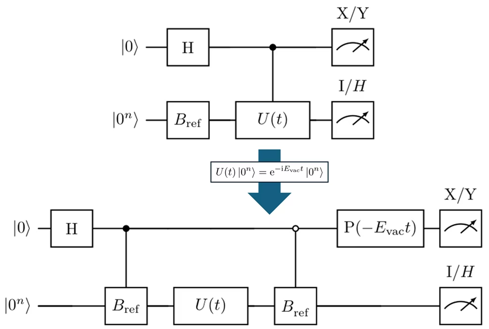
Aici, $B_{\rm ref}$ pregătește starea de referință, $B_{\rm ref}|0^n\rangle = |\psi_{0}\rangle$.

În loc să pregătim mai întâi $\frac{1}{\sqrt{2}}(|0\rangle+|1\rangle)|\psi_0\rangle$ și apoi să aplicăm $U(t)$ doar pe ramura $|1\rangle$, circuitul pregătește direct cele două ramuri ca

$$\begin{equation*} |0\rangle|\psi_0\rangle \quad \text{and} \quad |1\rangle|\psi_d\rangle , \end{equation*}$$

where

$$\begin{equation*} |\psi_d\rangle = U(d\Delta t)|\psi_0\rangle . \end{equation*}$$

Circuitul aplică mai întâi o poartă Hadamard asupra ancilei și pregătește starea de referință doar pe ramura $|1\rangle$:

$$\begin{equation*} |0\rangle |0^n\rangle \longrightarrow \frac{|0\rangle |0^n\rangle + |1\rangle B_{\rm ref}|0^n\rangle}{\sqrt{2}} = \frac{|0\rangle |0^n\rangle + |1\rangle |\psi_0\rangle}{\sqrt{2}} . \end{equation*}$$

Apoi operatorul de evoluție temporală necontrolat este aplicat ambelor ramuri:

$$\begin{equation*} \frac{|0\rangle |0^n\rangle + |1\rangle |\psi_0\rangle}{\sqrt{2}} \longrightarrow \frac{|0\rangle U(t)|0^n\rangle + |1\rangle U(t)|\psi_0\rangle}{\sqrt{2}} . \end{equation*}$$

Deoarece Hamiltonianul păstrează numărul de excitații, putem vedea că $|0^n\rangle$ este starea sa proprie, și astfel operatorul de evoluție acumulează doar o fază sub Hamiltonian:

$$\begin{equation*} U(t)|0^n\rangle = e^{-iE_{\rm vac}t}|0^n\rangle . \end{equation*}$$

Therefore,

$$\begin{equation*} \frac{|0\rangle U(t)|0^n\rangle + |1\rangle U(t)|\psi_0\rangle}{\sqrt{2}} = \frac{e^{-iE_{\rm vac}t}|0\rangle |0^n\rangle + |1\rangle U(t)|\psi_0\rangle}{\sqrt{2}} . \end{equation*}$$

În continuare, $B_{\rm ref}$ este aplicat doar pe ramura $|0\rangle$.

$$\begin{equation*} \frac{e^{-iE_{\rm vac}t}|0\rangle |\psi_0\rangle + |1\rangle U(t)|\psi_0\rangle}{\sqrt{2}} . \end{equation*}$$

În acest punct, cele două ramuri au o fază relativă suplimentară. Pentru a o elimina, aplicăm poarta de fază a ancilei

$$\begin{equation*} P(-E_{\rm vac}t) = \begin{pmatrix} 1 & 0 \\ 0 & e^{-iE_{\rm vac}t} \end{pmatrix}. \end{equation*}$$

Aceasta transformă starea astfel

$$\begin{equation*} \frac{e^{-iE_{\rm vac}t}|0\rangle |\psi_0\rangle + |1\rangle U(t)|\psi_0\rangle}{\sqrt{2}} \longrightarrow \frac{e^{-iE_{\rm vac}t}|0\rangle |\psi_0\rangle + e^{-iE_{\rm vac}t}|1\rangle U(t)|\psi_0\rangle}{\sqrt{2}} . \end{equation*}$$

Astfel, până la o fază globală irelevantă, am pregătit în final

$$\begin{equation*} |\Phi_{0d}\rangle = \frac{ |0\rangle|\psi_0\rangle + |1\rangle U(t)|\psi_0\rangle }{\sqrt{2}} . \end{equation*}$$

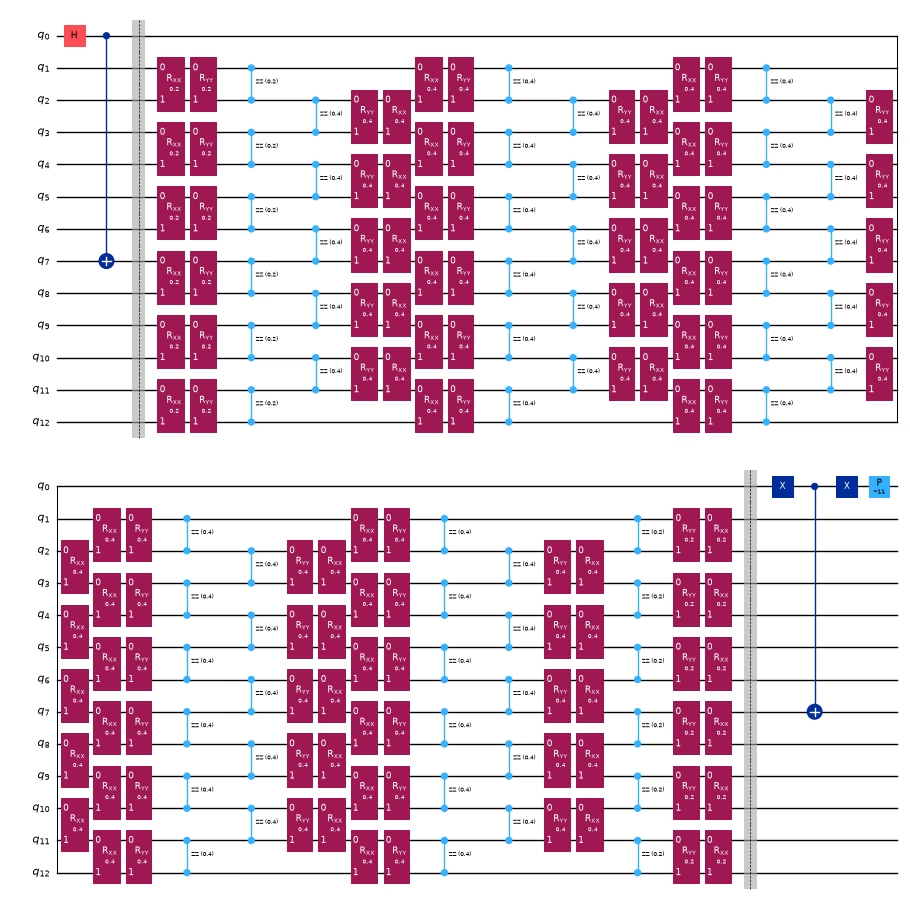
În următorul bloc de cod, implementăm acest circuit fără control.

controlled_extended_swap_test = extended_swap_test

# Reuse the ordering and synthesis rule selected by the comparison above.
evol_gate_optimized = PauliEvolutionGate(
    hamiltonian_for_synthesis,
    time=t,
    synthesis=SuzukiTrotter(order=2, reps=num_trotter_steps),
)

uncontrolled_evolution = QuantumCircuit(num_qubits, name="U_ST2(t)")
uncontrolled_evolution.append(evol_gate_optimized, range(num_qubits))

controlled_state_prep = QuantumCircuit(num_qubits + 1, name="C-Prep")
for q, bit in enumerate(reversed(ref_bitstring)):
    if bit == "1":
        controlled_state_prep.cx(ancilla, system_qubits[q])

vacuum_bitstring = "0" * num_qubits
vacuum_energy = basis_state_expectation_sparse(hamiltonian, "0" * num_qubits)

optimized_extended_swap_test = QuantumCircuit(num_qubits + 1)
optimized_extended_swap_test.h(ancilla)

# Prepare |psi_ref> only on the |1> branch.
optimized_extended_swap_test.compose(controlled_state_prep, inplace=True)
optimized_extended_swap_test.barrier()

# Apply the Trotterized time evolution without control.
optimized_extended_swap_test.compose(
    uncontrolled_evolution,
    qubits=system_qubits,
    inplace=True,
)
optimized_extended_swap_test.barrier()

# Map |0>|0...0> to |0>|psi_ref>, leaving the |1> branch unchanged.
optimized_extended_swap_test.x(ancilla)
optimized_extended_swap_test.compose(controlled_state_prep, inplace=True)
optimized_extended_swap_test.x(ancilla)

# Cancel the known vacuum phase so that the same X/Y observables can be used.
optimized_extended_swap_test.p(-vacuum_energy * t, ancilla)
optimized_extended_swap_test = simple_transpilation(
    optimized_extended_swap_test
)

print(f"Vacuum energy E_vac = {vacuum_energy:.1f}")
display(
    optimized_extended_swap_test.assign_parameters({t: 1.0}).draw(
        "mpl", scale=0.5, fold=26
    )
)

Vacuum energy E_vac = 11.0+0.0j

Transpilarea

Acum, transpilăm circuitele controlate și fără control pentru a deveni executabile pe hardware. Să comparăm rezultatul circuitelor transpilate.

pass_manager = generate_preset_pass_manager(
    backend=backend,
    optimization_level=3,
)

isa_controlled_extended_swap_test = pass_manager.run(
    controlled_extended_swap_test
)

pass_manager = generate_preset_pass_manager(
    backend=backend, optimization_level=3, routing_method="none"
)
isa_optimized_extended_swap_test = pass_manager.run(
    optimized_extended_swap_test
)

transpilation_result = [
    {
        "label": "abstract controlled U(t)",
        **summarize_circuit(isa_controlled_extended_swap_test),
    },
    {
        "label": "optimized non-controlled U(t)",
        **summarize_circuit(isa_optimized_extended_swap_test),
    },
]

display(pd.DataFrame(transpilation_result))

def filter_qubits_from_layout(layout):
    q_layout = Layout(
        {
            physical: virtual
            for physical, virtual in layout.get_physical_bits().items()
            if virtual._register.name == "q"
        }
    )
    return q_layout

print(
    filter_qubits_from_layout(
        isa_optimized_extended_swap_test.layout.initial_layout
    )
)

isa_observables = [
    op.apply_layout(isa_optimized_extended_swap_test.layout)
    for op in observables
]

label  depth   size  2q gates  2q depth
0       abstract controlled U(t)  15457  23786      4686      4580
1  optimized non-controlled U(t)    261   1716       307        57

Layout({
18: <Qubit register=(13, "q"), index=0>,
5: <Qubit register=(13, "q"), index=1>,
6: <Qubit register=(13, "q"), index=2>,
7: <Qubit register=(13, "q"), index=3>,
8: <Qubit register=(13, "q"), index=4>,
9: <Qubit register=(13, "q"), index=5>,
10: <Qubit register=(13, "q"), index=6>,
11: <Qubit register=(13, "q"), index=7>,
12: <Qubit register=(13, "q"), index=8>,
13: <Qubit register=(13, "q"), index=9>,
14: <Qubit register=(13, "q"), index=10>,
15: <Qubit register=(13, "q"), index=11>,
19: <Qubit register=(13, "q"), index=12>
})

Pasul 3: Execuție folosind primitivele Qiskit

Următorul pas este să transmitem același circuit parametrizat pentru mai multe valori ale $d$. Pentru fiecare $d$, estimăm patru valori de așteptare: $X\otimes I$, $Y\otimes I$, $X\otimes (H-T)$ și $Y\otimes (H-T)$. Aceste patru numere sunt apoi combinate în elementele complexe de pe primul rând $\mathcal{S}_{0d}$ și $\mathcal{H}_{0d}$.

Aici, $\mathcal{S}_{00}=1$ și $\mathcal{H}_{00}=\langle\psi_{0}|(H-T)|\psi_{0}\rangle=\langle\psi_{0}|H|\psi_{0}\rangle-\tau$ pot fi calculate clasic deoarece $\lvert\psi_0\rangle$ este rar, deci omitem cazul $d=0$.

pub_list = []
d_values = list(range(1, krylov_dim))

# Exact local statevector estimator.
estimator = StatevectorEstimator()

# We use the circuit before the transpilation for the local simulator,
# but we will use the transpiled circuit for the real backend.
for d in d_values:
    parameter_values = [d * dt]

    for ob in observables:
        pub_list.append(
            (
                optimized_extended_swap_test,
                ob,
                parameter_values,
            )
        )

job = estimator.run(pub_list)

# Local PrimitiveJob does not provide Runtime-style job inputs,
# so preserve the inputs directly.
inputs = pub_list
result = job.result()

print(f"Number of Krylov basis states: r = {len(d_values)}")
print(f"Number of PUBs: {len(pub_list)}")
print(f"Each d uses observables: {observable_labels}")

Number of Krylov basis states: r = 9
Number of PUBs: 36
Each d uses observables: ['Re S_0d', 'Im S_0d', 'Re shifted H_0d', 'Im shifted H_0d']

Pasul 4: Post-procesare și returnarea rezultatului în formatul clasic dorit

După estimarea matricelor proiectate, regularizăm și rezolvăm GEVP

$$\begin{equation*} \mathcal{H}\mathbf{c} = E\mathcal{S}\mathbf{c}. \end{equation*}$$

Cea mai mică valoare proprie generalizată dă estimarea KQD a energiei stării fundamentale.

h_shifted_row_est = np.zeros(krylov_dim, dtype=complex)
s_row_est = np.zeros(krylov_dim, dtype=complex)

h_shifted_row_est[0] = ref_energy - shift_tau
s_row_est[0] = 1.0

for idx, (pub_input, pub_result) in enumerate(zip(inputs, result)):
    d_index, obs_index = divmod(idx, len(observables))
    ev = np.asarray(pub_result.data.evs).reshape(-1)[0]
    std = np.asarray(pub_result.data.stds).reshape(-1)[0]

    if obs_index == 0:
        s_row_est[d_index + 1] = ev
    elif obs_index == 1:
        s_row_est[d_index + 1] += 1j * ev
    elif obs_index == 2:
        h_shifted_row_est[d_index + 1] = ev
    elif obs_index == 3:
        h_shifted_row_est[d_index + 1] += 1j * ev

# H_0d = shifted_H_0d + tau * S_0d.
h_row_est = h_shifted_row_est + shift_tau * s_row_est

h_matrix_est = la.toeplitz(h_row_est.conj(), h_row_est)
s_matrix_est = la.toeplitz(s_row_est.conj(), s_row_est)

s_eigvals = la.eigvalsh(0.5 * (s_matrix_est + s_matrix_est.conj().T))
positive_s_eigvals = s_eigvals[s_eigvals > 1e-12]
s_condition_number = (
    positive_s_eigvals[-1] / positive_s_eigvals[0]
    if len(positive_s_eigvals) > 0
    else np.inf
)

with np.printoptions(precision=3, suppress=True):
    print("Estimated first row of S:")
    print(s_row_est)
    print()
    print("Estimated first row of H:")
    print(h_row_est)
    print()
    print("Eigenvalues of the estimated overlap matrix S:")
    print(s_eigvals)
    print(f"Condition number above 1e-12: {s_condition_number:.3e}")
    print()

Estimated first row of S:
[ 1.   +0.j     0.758-0.596j  0.203-0.836j -0.291-0.636j -0.444-0.229j
 -0.276+0.053j -0.044+0.051j  0.006-0.121j -0.155-0.218j -0.345-0.101j]

Estimated first row of H:
[ 7.   +0.j     4.842-4.76j   0.044-6.185j -3.791-3.653j -4.137+0.39j
 -1.495+2.654j  1.331+1.777j  1.85 -0.763j -0.032-2.278j -2.222-1.372j]

Eigenvalues of the estimated overlap matrix S:
[-0.     0.     0.     0.     0.     0.     0.01   0.355  3.526  6.109]
Condition number above 1e-12: 1.904e+12

Acum rezolvăm problema generalizată de valori proprii folosind matricele reconstruite din estimările circuitului. Într-un calcul ideal de stare vectorială cu evoluție exactă în timp real, aceasta ar trebui să reproducă rezultatul proiectat exact. În practică, abaterile pot proveni din Trotterizare, eroarea de eșantionare și instabilitatea numerică a matricei de suprapunere.

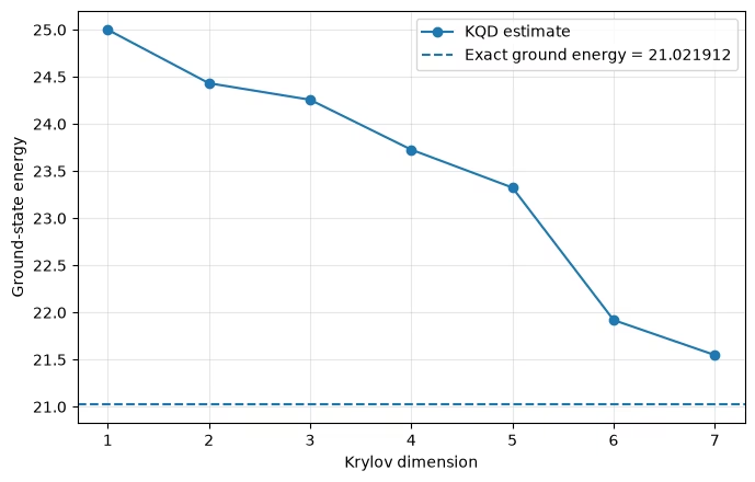
Observăm cum converge energia pe măsură ce creștem dimensiunea subspațiului Krylov.

exact_evals = diagonalize_single_1_subspace(hamiltonian)
exact_ground = min(exact_evals)
print("exact ground state energy:  ", exact_ground)

threshold = 1e-12
energy_convergence = []

for r in range(1, krylov_dim + 1):
    energy_est_kqd, coeffs_est, retained_est = solve_thresholded_gevp(
        h_matrix_est[:r, :r],
        s_matrix_est[:r, :r],
        threshold=threshold,
    )
    energy_convergence.append(energy_est_kqd)
    print(
        f"Krylov ground state energy (dim={r}, retained={retained_est}): ",
        energy_est_kqd,
    )

exact ground state energy:   3.136296694843727
Krylov ground state energy (dim=1, retained=1):  7.0
Krylov ground state energy (dim=2, retained=2):  4.184510657551266
Krylov ground state energy (dim=3, retained=3):  3.5539074630394136
Krylov ground state energy (dim=4, retained=4):  3.3366270761341044
Krylov ground state energy (dim=5, retained=5):  3.252017453225087
Krylov ground state energy (dim=6, retained=6):  3.2300275138879186
Krylov ground state energy (dim=7, retained=7):  3.2299154099085685
Krylov ground state energy (dim=8, retained=7):  3.2298063744216776
Krylov ground state energy (dim=9, retained=7):  3.2296778282872456
Krylov ground state energy (dim=10, retained=8):  3.223647515867734

def plot_energy_convergence(energy_convergence, exact_ground, krylov_dim):
    fig, ax = plt.subplots(figsize=(7, 4.5))

    ax.plot(
        range(1, krylov_dim + 1),
        energy_convergence,
        marker="o",
        label="KQD estimate",
    )

    ax.axhline(
        exact_ground,
        linestyle="--",
        label=f"Exact ground energy = {exact_ground:.6f}",
    )

    ax.set_xlabel("Krylov dimension")
    ax.set_ylabel("Ground-state energy")
    ax.grid(True, alpha=0.3)
    ax.legend()
    plt.tight_layout()
    plt.show()

plot_energy_convergence(energy_convergence, exact_ground, krylov_dim)

Exemplu de hardware la scară mare

Secțiunea anterioară a folosit un model de 12 qubiți, astfel încât simularea stării vectoriale să poată fi folosită ca diagnostic. Acum extindem același flux de lucru KQD la un lanț Heisenberg cu 30 de qubiți și pregătim sarcina de lucru pentru execuție pe hardware IBM Quantum.

Pașii 1-4 comprimați într-un singur bloc de cod

Acum reunim toate aceste detalii într-un flux de lucru unic la o scară mai mare, care este apoi rulat pe hardware-ul nostru cuantic real. În această secțiune, aplicăm setări realiste de atenuare a erorilor pentru a îmbunătăți fiabilitatea rezultatelor. Deoarece elementele matriceale corespunzătoare diferitelor valori ale $d$ pot fi evaluate în paralel, folosim modul Batch pentru a le executa eficient.

# -------------------------Step 1-------------------------

# Map the classical problem to quantum circuits and observables.
# Problem and KQD parameters.
large_num_qubits = 30
large_krylov_dim = 7
large_num_trotter_steps = 3
large_dt = np.pi / (3 * (large_num_qubits - 1))
large_t = Parameter("t_large")

# Use a single excitation near the center of the chain.
large_excitation_qubit = large_num_qubits // 2
large_ref_label = ["0"] * large_num_qubits
large_ref_label[large_num_qubits - 1 - large_excitation_qubit] = "1"
large_ref_bitstring = "".join(large_ref_label)

# Use the ordering and product formula selected in the preceding section.
large_hamiltonian = make_heisenberg_hamiltonian_ordered(
    large_num_qubits,
    ordering="even-odd edge-grouped",
    coupling=1.0,
)
large_ref_energy = float(
    np.real(
        basis_state_expectation_sparse(large_hamiltonian, large_ref_bitstring)
    )
)
large_vacuum_energy = float(
    np.real(
        basis_state_expectation_sparse(
            large_hamiltonian, "0" * large_num_qubits
        )
    )
)

large_evolution_gate = PauliEvolutionGate(
    large_hamiltonian,
    time=large_t,
    synthesis=SuzukiTrotter(order=2, reps=large_num_trotter_steps),
)
large_uncontrolled_evolution = QuantumCircuit(
    large_num_qubits,
    name="U_ST2_large(t)",
)
large_uncontrolled_evolution.append(
    large_evolution_gate,
    range(large_num_qubits),
)

# Build the control-free extended-swap-test circuit.
large_ancilla = 0
large_system_qubits = list(range(1, large_num_qubits + 1))

large_controlled_state_prep = QuantumCircuit(
    large_num_qubits + 1,
    name="C-Prep-large",
)
large_controlled_state_prep.cx(
    large_ancilla,
    large_system_qubits[large_excitation_qubit],
)

large_extended_swap_test = QuantumCircuit(large_num_qubits + 1)
large_extended_swap_test.h(large_ancilla)
large_extended_swap_test.compose(large_controlled_state_prep, inplace=True)
large_extended_swap_test.compose(
    large_uncontrolled_evolution,
    qubits=large_system_qubits,
    inplace=True,
)
large_extended_swap_test.x(large_ancilla)
large_extended_swap_test.compose(
    large_controlled_state_prep.inverse(),
    inplace=True,
)
large_extended_swap_test.x(large_ancilla)
large_extended_swap_test.p(
    -large_vacuum_energy * large_t,
    large_ancilla,
)

# Reuse the Hamiltonian-shifting construction from the preceding section.
(
    large_obs_x_shifted_hamiltonian,
    large_obs_y_shifted_hamiltonian,
    large_shift_tau,
) = make_reduced_heisenberg_observables(large_ref_bitstring)

large_observables = [
    SparsePauliOp("I" * large_num_qubits + "X"),
    SparsePauliOp("I" * large_num_qubits + "Y"),
    large_obs_x_shifted_hamiltonian,
    large_obs_y_shifted_hamiltonian,
]
large_observable_labels = [
    "Re S_0d",
    "Im S_0d",
    "Re shifted H_0d",
    "Im shifted H_0d",
]

# -------------------------Step 2-------------------------

# Optimize the problem for quantum execution.
# Select a real backend and transpile the parameterized circuit to ISA form.
large_backend = service.backend("ibm_boston")
large_pass_manager = generate_preset_pass_manager(
    backend=large_backend, optimization_level=3, routing_method="none"
)
large_isa_circuit = large_pass_manager.run(large_extended_swap_test)
large_isa_observables = [
    observable.apply_layout(large_isa_circuit.layout)
    for observable in large_observables
]

large_two_qubit_gate_count = sum(
    instruction.operation.num_qubits == 2
    for instruction in large_isa_circuit.data
)

print(f"Backend: {large_backend.name}")
print(f"System qubits: {large_num_qubits}")
print(f"Total circuit qubits: {large_isa_circuit.num_qubits}")
print(f"Krylov dimension: {large_krylov_dim}")
print(f"Time step: {large_dt:.6f}")
print(f"Shift tau: {large_shift_tau}")
print(f"ISA circuit depth: {large_isa_circuit.depth()}")
print(f"ISA two-qubit gates: {large_two_qubit_gate_count}")
print(
    f"ISA two-qubit depth: {large_isa_circuit.depth(lambda x: x[0].num_qubits == 2)}"
)

# -------------------------Step 3-------------------------

# Execute on quantum hardware with Qiskit Runtime primitives.
# Submit one job per d, with all four observables in that job.
large_d_values = list(range(1, large_krylov_dim))
retrieve_batch_id = None
large_jobs = []

if retrieve_batch_id is None:
    large_estimator_options = {
        "default_shots": 8192,
        "dynamical_decoupling": {
            "enable": True,
            "sequence_type": "XpXm",
        },
        "resilience": {
            "measure_mitigation": True,
            "measure_noise_learning": {
                "num_randomizations": 32,
                "shots_per_randomization": 256,
            },
            "layer_noise_learning": {
                "max_layers_to_learn": 4,
                "layer_pair_depths": [0, 1, 2, 4, 16, 32],
                "num_randomizations": 32,
                "shots_per_randomization": 128,
            },
            "zne_mitigation": True,
            "zne": {
                "amplifier": "pea",
                "noise_factors": [1.0, 1.5, 2.0],
                "extrapolator": ("exponential", "linear"),
            },
        },
        "twirling": {
            "enable_gates": True,
            "enable_measure": True,
            "num_randomizations": 32,
            "shots_per_randomization": 256,
            "strategy": "active-accum",
        },
    }

    with Batch(backend=large_backend) as large_batch:
        large_batch_id = large_batch.session_id
        large_estimator = EstimatorV2(
            mode=large_batch,
            options=large_estimator_options,
        )
        # Krylov quantum diagonalization of lattice Hamiltonians -> TUT_KQDOLH.
        large_estimator.options.environment.job_tags = ["TUT_KQDOLH"]

        for d in large_d_values:
            parameter_values = [d * large_dt]
            pubs_for_d = [
                (large_isa_circuit, observable, parameter_values)
                for observable in large_isa_observables
            ]
            job = large_estimator.run(pubs_for_d)
            large_jobs.append(job)
            print(
                f"Submitted d={d}: job_id={job.job_id()}, "
                f"PUBs={len(pubs_for_d)}"
            )

    print(f"Batch ID: {large_batch_id}")
else:
    large_batch_id = retrieve_batch_id
    large_jobs = service.jobs(
        session_id=large_batch_id,
        limit=None,
        descending=False,
    )

large_job_ids_by_d = {
    d: job.job_id() for d, job in zip(large_d_values, large_jobs)
}
print(f"Job IDs by d: {large_job_ids_by_d}")

# -------------------------Step 4-------------------------

# Post-process the quantum results and solve the classical GEVP.
# Reconstruct the first rows of S and the shifted Hamiltonian matrix.
large_s_row_est = np.zeros(large_krylov_dim, dtype=complex)
large_h_shifted_row_est = np.zeros(large_krylov_dim, dtype=complex)
large_s_row_est[0] = 1.0
large_h_shifted_row_est[0] = large_ref_energy - large_shift_tau

for d, job in zip(large_d_values, large_jobs):
    job_result = job.result()

    if len(job_result) != len(large_observables):
        raise RuntimeError(
            f"Expected {len(large_observables)} PUB results for d={d}, "
            f"but received {len(job_result)}."
        )

    expectation_values = [
        np.asarray(pub_result.data.evs).reshape(-1)[0]
        for pub_result in job_result
    ]

    large_s_row_est[d] = expectation_values[0] + 1j * expectation_values[1]
    large_h_shifted_row_est[d] = (
        expectation_values[2] + 1j * expectation_values[3]
    )

# H_0d = shifted_H_0d + tau * S_0d.
large_h_row_est = large_h_shifted_row_est + large_shift_tau * large_s_row_est

large_s_matrix_est = la.toeplitz(
    large_s_row_est.conj(),
    large_s_row_est,
)
large_h_matrix_est = la.toeplitz(
    large_h_row_est.conj(),
    large_h_row_est,
)

large_exact_gnd = min(diagonalize_single_1_subspace(large_hamiltonian))

large_energy_convergence = []

with np.printoptions(precision=5, suppress=True):
    print("Estimated first row of S:")
    print(large_s_row_est)
    print("Estimated first row of H:")
    print(large_h_row_est)
    print("exact ground state energy:  ", large_exact_gnd)

    for r in range(1, large_krylov_dim + 1):
        energy_est_kqd, coeffs_est, retained_est = solve_thresholded_gevp(
            large_h_matrix_est[:r, :r],
            large_s_matrix_est[:r, :r],
            threshold=5e-2,
        )
        large_energy_convergence.append(energy_est_kqd)
        print(
            f"Krylov ground state energy (dim={r}, retained={retained_est}): ",
            energy_est_kqd,
        )

plot_energy_convergence(
    large_energy_convergence, large_exact_gnd, large_krylov_dim
)

Backend: ibm_boston
System qubits: 30
Total circuit qubits: 156
Krylov dimension: 7
Time step: 0.036110
Shift tau: 25.0
ISA circuit depth: 219
ISA two-qubit gates: 728
ISA two-qubit depth: 52
Job IDs by d: {1: 'd9fl4p4jeosc73fk4dg0', 2: 'd9fl4pineu4c739poecg', 3: 'd9fl4q2neu4c739poedg', 4: 'd9fl4qhhtsac739fjgn0', 5: 'd9fl4r4jeosc73fk4dhg', 6: 'd9fl4rkjeosc73fk4dj0'}
Estimated first row of S:
[ 1.     +0.j       0.42055-0.65466j -0.17883-0.73125j -0.64523-0.31601j
 -0.70781+0.55574j -0.02467+0.70525j  0.59301+0.55602j]
Estimated first row of H:
[ 25.      +0.j       10.3419 -16.5586j   -5.017  -18.03933j
 -16.44797 -6.98173j -17.17081+14.84502j   0.62722+17.81196j
  15.68886+12.74875j]
exact ground state energy:   21.021912418526902
Krylov ground state energy (dim=1, retained=1):  25.0
Krylov ground state energy (dim=2, retained=2):  24.432409110686205
Krylov ground state energy (dim=3, retained=3):  24.256856893278556
Krylov ground state energy (dim=4, retained=4):  23.727409826799715
Krylov ground state energy (dim=5, retained=4):  23.324720470780864
Krylov ground state energy (dim=6, retained=5):  21.91957579005085
Krylov ground state energy (dim=7, retained=5):  21.548331214122644

Anexă: Perspectiva funcției Hamiltoniene (filtru spectral)

Fluxul de lucru principal a prezentat KQD în mod operațional: construirea unei baze Krylov din stări evoluate în timp real, estimarea matricelor proiectate $\mathcal{H}$ și $\mathcal{S}$, și rezolvarea GEVP. Această anexă revizitează același calcul dintr-un unghi complementar care explică de ce funcționează KQD: perspectiva funcției Hamiltoniene, sau a filtrului spectral [3], [5]. Aceasta reutilizează modelul de 12 qubiți, pasul de timp $\Delta t$ și soluția Krylov deja obținută mai sus; nu este necesară nicio execuție nouă de circuit.

Starea de referință ca distribuție de energie

Fie Hamiltonianul având descompunerea proprie

$$\begin{equation*} H=\sum_{m} E_m\,|E_m\rangle\!\langle E_m|, \qquad E_0\le E_1\le\cdots, \end{equation*}$$

cu stările proprii de energie $|E_m\rangle$. Orice stare de referință poate fi extinsă în această bază proprie,

$$\begin{equation*} |\psi_{0}\rangle=\sum_m a_m\,|E_m\rangle, \qquad a_m=\langle E_m|\psi_{0}\rangle, \end{equation*}$$

astfel încât poartă o pondere spectrală $p_m=|a_m|^2$ la fiecare energie $E_m$. Energia de referință este media acestei distribuții, $\langle H\rangle_{0}=\sum_m p_m E_m$.

Descompunerea proprie a unui Hamiltonian general de $n$ qubiți este costisitoare exponențial, deci această imagine este doar un diagnostic, care nu face parte din algoritm. Aici, totuși, o putem calcula ieftin pentru aceeași problemă cu $n=12$: Hamiltonianul Heisenberg conservă numărul total de excitații, iar referința $|000001000000\rangle$ poartă o singură excitație, deci întregul său conținut spectral se află în subspațiul cu o singură excitație, a cărui dimensiune crește doar liniar cu $n$. Prin urmare, reutilizăm blocul exact cu o singură excitație (deja folosit mai sus ca reper) și citim distribuția de referință $\{(E_m, p_m)\}$ în interiorul acelui subspațiu.

# Exact single-excitation-subspace decomposition of the reference state.
# This reuses make_heisenberg_hamiltonian / _basis_state_transition_amplitude_sparse
# and the n=12 `hamiltonian` and `ref_bitstring` defined in the small-scale example.
single_excitation_states = [1 << k for k in range(num_qubits)]

h_single = np.array(
    [
        [
            _basis_state_transition_amplitude_sparse(hamiltonian, bra, ket)
            for ket in single_excitation_states
        ]
        for bra in single_excitation_states
    ]
)
h_single = 0.5 * (h_single + h_single.conj().T)

subspace_evals, subspace_evecs = la.eigh(h_single)
subspace_evals = np.real(subspace_evals)

# Reference-state coordinates inside the single-excitation subspace.
ref_position = single_excitation_states.index(int(ref_bitstring, 2))
ref_in_subspace = np.zeros(num_qubits, dtype=complex)
ref_in_subspace[ref_position] = 1.0

# Amplitudes and spectral weights of the reference in the energy eigenbasis.
ref_eigen_amplitudes = subspace_evecs.conj().T @ ref_in_subspace
ref_spectral_weights = np.abs(ref_eigen_amplitudes) ** 2

print(f"Single-excitation subspace dimension: {num_qubits}")
print(f"Subspace ground-state energy:         {subspace_evals[0]:.6f}")
print(
    f"Reference energy (sum p_m E_m):       {np.sum(ref_spectral_weights * subspace_evals):.6f}"
)
print(f"Reference weight on subspace ground:  {ref_spectral_weights[0]:.6f}")

Single-excitation subspace dimension: 12
Subspace ground-state energy:         3.136297
Reference energy (sum p_m E_m):       7.000000
Reference weight on subspace ground:  0.163827

KQD învață un filtru care remodelează această distribuție

O funcție Hamiltoniană $f(H)$ este definită prin calcul spectral,

$$\begin{equation*} f(H)=\sum_m f(E_m)\,|E_m\rangle\!\langle E_m|, \end{equation*}$$

sau, cu alte cuvinte, o sumă ponderată de proiectori proprii. Aplicarea ei asupra referinței remodelează fiecare amplitudine spectrală, $a_m \to a_m f(E_m)$:

$$\begin{equation*} f(H)\,|\psi_{0}\rangle=\sum_m a_m\,f(E_m)\,|E_m\rangle . \end{equation*}$$

Dacă $f$ ar fi puternic concentrată la energia cea mai joasă ($f(E_0)=1$ și $f(E_m)\approx 0$ în rest), atunci $f(H)$ ar acționa ca un proiector pe starea fundamentală, iar ieșirea normalizată ar fi (aproape) starea fundamentală. Prin urmare, un filtru spectral trece-jos bun în energie este exact ceea ce ne dorim.

KQD nu prescrie $f$ în avans. În schimb, extinde filtrul în baza evoluției în timp real,

$$\begin{equation*} f_{\rm KQD}(E)=\sum_{\ell=0}^{r-1} c_\ell\, e^{-i\ell\Delta t E}, \end{equation*}$$

o funcție trigonometrică a energiei ale cărei coeficienți $\{c_\ell\}$ sunt exact vectorul propriu GEVP rezolvat mai sus. Minimizarea raportului Rayleigh $\mathbf{c}^\dagger\mathcal{H}\mathbf{c}/\mathbf{c}^\dagger\mathcal{S}\mathbf{c}$ este așadar echivalentă cu învățarea filtrului care suprimă cel mai bine ponderea stărilor excitate ale referinței. O dimensiune Krylov $r$ mai mare oferă filtrului mai multe grade de libertate și un vârf mai ascuțit la energia stării fundamentale.

Funcția ajutătoare de mai jos evaluează acest filtru învățat pe o axă de energie; apoi îl aplicăm distribuției de referință obținute mai sus.

def trigonometric_krylov_filter(
    coeffs: np.ndarray,
    energies: np.ndarray,
    time_step: float,
) -> np.ndarray:
    """Evaluate the learned Krylov filter f(E) = sum_l c_l exp(-i l dt E)."""
    values = np.zeros_like(energies, dtype=complex)
    for ell, coeff in enumerate(coeffs):
        values += coeff * np.exp(-1j * ell * time_step * energies)
    return values

def filtered_spectral_weights(
    weights: np.ndarray,
    filter_values: np.ndarray,
) -> np.ndarray:
    """Reshape spectral weights by |f(E)|^2 and renormalize."""
    reshaped = weights * np.abs(filter_values) ** 2
    return reshaped / np.sum(reshaped)

# Recover the KQD coefficients from the already-estimated projected matrices.
# The shift only moves H by tau * S, so it does not change the GEVP eigenvector;
# we solve at the full Krylov dimension used in the small-scale example.
_, kqd_coeffs, _ = solve_thresholded_gevp(
    h_matrix_est,
    s_matrix_est,
    threshold=1e-12,
)

filter_on_spectrum = trigonometric_krylov_filter(
    kqd_coeffs, subspace_evals, dt
)
filtered_weights = filtered_spectral_weights(
    ref_spectral_weights, filter_on_spectrum
)

print(f"Ground-state overlap  (reference): {ref_spectral_weights[0]:.4f}")
print(f"Ground-state overlap  (filtered):  {filtered_weights[0]:.4f}")
print(
    f"Mean energy           (reference): {np.sum(ref_spectral_weights * subspace_evals):.6f}"
)
print(
    f"Mean energy           (filtered):  {np.sum(filtered_weights * subspace_evals):.6f}"
)

Ground-state overlap  (reference): 0.1638
Ground-state overlap  (filtered):  0.9638
Mean energy           (reference): 7.000000
Mean energy           (filtered):  3.164503

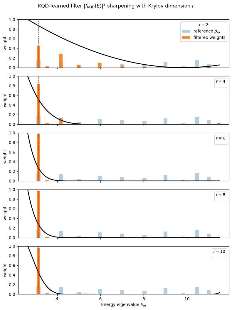
Vizualizarea filtrului și a flexibilității sale

Arătăm mai întâi filtrul învățat la dimensiunea Krylov completă folosită mai sus, apoi urmărim cum se ascute pe măsură ce dimensiunea $r$ crește.

Barele arată ponderile spectrale de referință $p_m$ (înainte) și ponderile filtrate $p_m|f_{\rm KQD}(E_m)|^2$ (după), împreună cu intensitatea filtrului învățat $|f_{\rm KQD}(E)|^2$ pe o axă de energie continuă. Filtrul concentrează ponderea pe cea mai joasă energie a subspațiului cu o singură excitație — aceeași energie la care a convergent estimarea KQD în exemplul la scară mică. Rețineți că aceasta este starea fundamentală în interiorul sectorului cu o singură excitație, care este ținta relevantă pentru această stare de referință care conservă excitația, nu starea fundamentală globală.

fig, ax = plt.subplots(figsize=(8, 4))

visible = (ref_spectral_weights > 1e-4) | (filtered_weights > 1e-4)
ax.bar(
    subspace_evals[visible],
    ref_spectral_weights[visible],
    width=0.18,
    alpha=0.45,
    label="reference $p_m$",
)
ax.bar(
    subspace_evals[visible],
    filtered_weights[visible],
    width=0.14,
    alpha=0.9,
    label=r"filtered $p_m\,|f_{\rm KQD}(E_m)|^2$",
)

energy_grid = np.linspace(
    subspace_evals.min() - 0.5, subspace_evals.max() + 0.5, 800
)
filter_intensity = (
    np.abs(trigonometric_krylov_filter(kqd_coeffs, energy_grid, dt)) ** 2
)
filter_intensity /= filter_intensity.max()
ax.plot(
    energy_grid,
    filter_intensity,
    color="k",
    linewidth=2,
    label=r"$|f_{\rm KQD}(E)|^2$ (normalized)",
)

ax.axvline(
    subspace_evals[0],
    color="C3",
    linestyle="--",
    linewidth=1,
    label="subspace ground energy",
)
ax.set_xlabel("Energy eigenvalue $E_m$")
ax.set_ylabel("Spectral weight")
ax.set_ylim(0, 1)
ax.legend(loc="upper right")
plt.tight_layout()
plt.show()

Creșterea dimensiunii Krylov: flexibilitatea funcției învățate

Reamintim că filtrul învățat este un polinom trigonometric în energie cu $r$ coeficienți,

$$\begin{equation*} f_{\rm KQD}(E)=\sum_{\ell=0}^{r-1} c_\ell\, e^{-i\ell\Delta t E}. \end{equation*}$$

Dimensiunea Krylov $r$ este exact numărul de coeficienți liberi, deci controlează flexibilitatea funcției. Un $r$ mic poate produce doar un filtru larg, care variază lin și lasă să se scurgă pondere în stările excitate de joasă energie; când $r$ crește, filtrul poate forma un vârf mai îngust la energia țintă și poate suprima mai agresiv ponderea rămasă a stărilor excitate. Aceasta este contrapartida în filtru spectral a convergenței energiei observate în exemplul la scară mică: pe măsură ce $r$ crește, distribuția filtrată se prăbușește pe starea fundamentală a subspațiului, iar energia estimată scade către aceasta.

Reutilizăm matricele proiectate deja estimate mai sus și pur și simplu rezolvăm GEVP la fiecare bloc principal $r\times r$, apoi evaluăm și reprezentăm grafic filtrul corespunzător.

# Sweep the Krylov dimension using the leading r x r blocks of the estimated matrices.
sweep_dims = [r for r in (2, 4, 6, 8, krylov_dim) if r <= krylov_dim]
sweep_dims = sorted(set(sweep_dims))

energy_grid = np.linspace(
    subspace_evals.min() - 0.5, subspace_evals.max() + 0.5, 800
)

sweep_cases = []
print(" r    retained    ground overlap    filtered energy")
print("--    --------    --------------    ---------------")
for r in sweep_dims:
    _, coeffs_r, retained_r = solve_thresholded_gevp(
        h_matrix_est[:r, :r],
        s_matrix_est[:r, :r],
        threshold=1e-12,
    )
    filter_on_spectrum_r = trigonometric_krylov_filter(
        coeffs_r, subspace_evals, dt
    )
    filtered_weights_r = filtered_spectral_weights(
        ref_spectral_weights, filter_on_spectrum_r
    )
    filtered_energy_r = float(np.sum(filtered_weights_r * subspace_evals))

    sweep_cases.append((r, coeffs_r, filtered_weights_r))
    print(
        f"{r:2d}    {retained_r:8d}    {filtered_weights_r[0]:14.4f}    {filtered_energy_r:15.6f}"
    )

print(f"\nSubspace ground-state energy (target): {subspace_evals[0]:.6f}")

# One panel per Krylov dimension: filtered spectrum (bars) + filter intensity (curve).
fig, axes = plt.subplots(
    len(sweep_cases),
    1,
    figsize=(8, 2.1 * len(sweep_cases)),
    sharex=True,
)
axes = np.atleast_1d(axes)

for idx, (ax, (r, coeffs_r, filtered_weights_r)) in enumerate(
    zip(axes, sweep_cases)
):
    visible = (ref_spectral_weights > 1e-4) | (filtered_weights_r > 1e-4)
    ax.bar(
        subspace_evals[visible],
        ref_spectral_weights[visible],
        width=0.18,
        alpha=0.35,
        color="C0",
        label="reference $p_m$" if idx == 0 else None,
    )
    ax.bar(
        subspace_evals[visible],
        filtered_weights_r[visible],
        width=0.14,
        alpha=0.9,
        color="C1",
        label="filtered weights" if idx == 0 else None,
    )

    filter_intensity_r = (
        np.abs(trigonometric_krylov_filter(coeffs_r, energy_grid, dt)) ** 2
    )
    filter_intensity_r /= filter_intensity_r.max()
    ax.plot(energy_grid, filter_intensity_r, color="k", linewidth=2)

    ax.axvline(subspace_evals[0], color="C3", linestyle="--", linewidth=1)
    ax.set_ylim(0, 1)
    ax.set_ylabel("weight")
    ax.legend(loc="upper right", title=f"$r={r}$")

axes[-1].set_xlabel("Energy eigenvalue $E_m$")
fig.suptitle(
    r"KQD-learned filter $|f_{\rm KQD}(E)|^2$ sharpening with Krylov dimension $r$",
    y=1.0,
)
fig.tight_layout()
plt.show()

r    retained    ground overlap    filtered energy
--    --------    --------------    ---------------
 2           2            0.4549           4.184510
 4           4            0.8373           3.310168
 6           6            0.9706           3.158100
 8           7            0.9701           3.158725
10           8            0.9638           3.164503

Subspace ground-state energy (target): 3.136297

Pași următori

Dacă acest material ți s-a părut interesant, s-ar putea să te intereseze următoarele resurse:

Recomandări

• Diagonalizare Krylov cuantică bazată pe eșantioane a unui model de rețea fermionic
• Estimarea energiei stării fundamentale a lanțului Heisenberg cu VQE
• Curs despre algoritmi de diagonalizare cuantică

Referințe

[1] E. N. Epperly, L. Lin, and Y. Nakatsukasa, A theory of quantum subspace diagonalization, SIAM Journal on Matrix Analysis and Applications 43, 1263-1290 (2022).

[2] N. Yoshioka, M. Amico, W. Kirby, et al., Diagonalization of large many-body Hamiltonians on a quantum processor, arXiv:2407.14431 (2024).

[3] R. M. Parrish și P. L. McMahon, Quantum filter diagonalization: quantum eigendecomposition without full quantum phase estimation, Physical Review Letters 122, 230401 (2019).

[4] G. Lee, S. Choi, J. Huh și A. F. Izmaylov, Efficient strategies for reducing sampling error in quantum Krylov subspace diagonalization, Digital Discovery 4, 954-969 (2025).

[5] G. Lee, M. Kang, J. Hong, S. Fomichev și J. Huh, Filtered Quantum Phase Estimation, arXiv:2510.04294 (2025).