Modelul Ising cu Câmp Transversal și Managementul Performanței Q-CTRL

Estimare de utilizare: 2 minute pe un procesor Heron r2. (NOTĂ: Aceasta este doar o estimare. Timpul tău de execuție poate varia.)

Fundal

Modelul Ising cu Câmp Transversal (TFIM) este important pentru studiul magnetismului cuantic și al tranzițiilor de fază. Acesta descrie un set de spini dispuși pe o rețea, unde fiecare spin interacționează cu vecinii săi și este, totodată, influențat de un câmp magnetic extern care generează fluctuații cuantice.

O abordare frecventă pentru a simula acest model este utilizarea descompunerii Trotter pentru a aproxima operatorul de evoluție temporală, construind circuite care alternează între rotații pe un singur Qubit și interacțiuni cu doi Qubiți. Cu toate acestea, această simulare pe hardware real este dificilă din cauza zgomotului și a decoherenței, ceea ce duce la abateri față de dinamica reală. Pentru a depăși această problemă, folosim instrumentele de suprimare a erorilor și management al performanței Fire Opal de la Q-CTRL, oferite ca o funcție Qiskit (vezi documentația Fire Opal). Fire Opal optimizează automat execuția circuitelor prin aplicarea decuplării dinamice, layout-ului avansat, rutării și altor tehnici de suprimare a erorilor, toate menite să reducă zgomotul. Datorită acestor îmbunătățiri, rezultatele hardware se aliniază mai bine cu simulările fără zgomot, putând astfel studia dinamica magnetizării TFIM cu o fidelitate mai mare.

În acest tutorial vom:

• Construi Hamiltonianul TFIM pe un graf de triunghiuri de spini conectate
• Simula evoluția temporală cu circuite Trotterizate la diferite adâncimi
• Calcula și vizualiza magnetizările pe un singur Qubit $\langle Z_i \rangle$ în timp
• Compara simulările de bază cu rezultatele obținute pe hardware real folosind managementul performanței Fire Opal de la Q-CTRL

Prezentare generală

Modelul Ising cu Câmp Transversal (TFIM) este un model de spini cuantici care surprinde caracteristicile esențiale ale tranzițiilor de fază cuantice. Hamiltonianul este definit astfel:

$$H = -J \sum_{i} Z_i Z_{i+1} - h \sum_{i} X_i$$

unde $Z_i$ și $X_i$ sunt operatori Pauli care acționează asupra Qubitului $i$, $J$ este intensitatea cuplajului dintre spini vecini, iar $h$ este intensitatea câmpului magnetic transversal. Primul termen reprezintă interacțiunile feromagnetice clasice, în timp ce al doilea introduce fluctuații cuantice prin câmpul transversal. Pentru a simula dinamica TFIM, se folosește o descompunere Trotter a operatorului de evoluție unitară $e^{-iHt}$, implementată prin straturi de porți RX și RZZ bazate pe un graf personalizat de triunghiuri de spini conectate. Simularea explorează modul în care magnetizarea $\langle Z \rangle$ evoluează odată cu creșterea numărului de pași Trotter.

Performanța implementării TFIM propuse este evaluată prin compararea simulărilor fără zgomot cu backend-urile cu zgomot. Funcțiile de execuție îmbunătățită și de suprimare a erorilor Fire Opal sunt utilizate pentru a atenua efectul zgomotului pe hardware real, oferind estimări mai fiabile ale observabilelor de spin, precum $\langle Z_i \rangle$ și corelatorii $\langle Z_i Z_j \rangle$.

Cerințe

Înainte de a începe acest tutorial, asigură-te că ai instalate următoarele:

• Qiskit SDK v1.4 sau mai recent, cu suport pentru vizualizare
• Qiskit Runtime v0.40 sau mai recent (pip install qiskit-ibm-runtime)
• Qiskit Functions Catalog v0.9.0 (pip install qiskit-ibm-catalog)
• Fire Opal SDK v9.0.2 sau mai recent (pip install fire-opal)
• Q-CTRL Visualizer v8.0.2 sau mai recent (pip install qctrl-visualizer)

Configurare

Mai întâi, autentifică-te folosind cheia ta API IBM Quantum. Apoi, selectează funcția Qiskit după cum urmează. (Acest cod presupune că ți-ai salvat deja contul în mediul local.)

# Added by doQumentation — required packages for this notebook
!pip install -q matplotlib networkx numpy qctrlvisualizer qiskit qiskit-aer qiskit-ibm-catalog qiskit-ibm-runtime

from qiskit.transpiler.preset_passmanagers import generate_preset_pass_manager
from qiskit import QuantumCircuit
from qiskit_ibm_catalog import QiskitFunctionsCatalog
from qiskit_ibm_runtime import QiskitRuntimeService
from qiskit_ibm_runtime import SamplerV2 as Sampler
from qiskit.quantum_info import SparsePauliOp
from qiskit_aer import AerSimulator

import numpy as np
import networkx as nx
import matplotlib.pyplot as plt
import qctrlvisualizer as qv

catalog = QiskitFunctionsCatalog(channel="ibm_quantum_platform")

# Access Function
perf_mgmt = catalog.load("q-ctrl/performance-management")

Pasul 1: Maparea intrărilor clasice la o problemă cuantică

Generarea grafului TFIM

Începem prin definirea rețelei de spini și a cuplajelor dintre aceștia. În acest tutorial, rețeaua este construită din triunghiuri conectate dispuse într-un lanț liniar. Fiecare triunghi constă din trei noduri conectate într-o buclă închisă, iar lanțul se formează prin legarea unui nod din fiecare triunghi de triunghiul anterior.

Funcția ajutătoare connected_triangles_adj_matrix construiește matricea de adiacență pentru această structură. Pentru un lanț de $n$ triunghiuri, graful rezultat conține $2n+1$ noduri.

def connected_triangles_adj_matrix(n):
    """
    Generate the adjacency matrix for 'n' connected triangles in a chain.
    """
    num_nodes = 2 * n + 1
    adj_matrix = np.zeros((num_nodes, num_nodes), dtype=int)

    for i in range(n):
        a, b, c = i * 2, i * 2 + 1, i * 2 + 2  # Nodes of the current triangle

        # Connect the three nodes in a triangle
        adj_matrix[a, b] = adj_matrix[b, a] = 1
        adj_matrix[b, c] = adj_matrix[c, b] = 1
        adj_matrix[a, c] = adj_matrix[c, a] = 1

        # If not the first triangle, connect to the previous triangle
        if i > 0:
            adj_matrix[a, a - 1] = adj_matrix[a - 1, a] = 1

    return adj_matrix

Pentru a vizualiza rețeaua definită, putem reprezenta grafic lanțul de triunghiuri conectate și eticheta fiecare nod. Funcția de mai jos construiește graful pentru un număr ales de triunghiuri și îl afișează.

def plot_triangle_chain(n, side=1.0):
    """
    Plot a horizontal chain of n equilateral triangles.
    Baseline: even nodes (0,2,4,...,2n) on y=0
    Apexes: odd nodes (1,3,5,...,2n-1) above the midpoint.
    """
    # Build graph
    A = connected_triangles_adj_matrix(n)
    G = nx.from_numpy_array(A)

    h = np.sqrt(3) / 2 * side
    pos = {}

    # Place baseline nodes
    for k in range(n + 1):
        pos[2 * k] = (k * side, 0.0)

    # Place apex nodes
    for k in range(n):
        x_left = pos[2 * k][0]
        x_right = pos[2 * k + 2][0]
        pos[2 * k + 1] = ((x_left + x_right) / 2, h)

    # Draw
    fig, ax = plt.subplots(figsize=(1.5 * n, 2.5))
    nx.draw(
        G,
        pos,
        ax=ax,
        with_labels=True,
        font_size=10,
        font_color="white",
        node_size=600,
        node_color=qv.QCTRL_STYLE_COLORS[0],
        edge_color="black",
        width=2,
    )
    ax.set_aspect("equal")
    ax.margins(0.2)
    plt.show()

    return G, pos

Pentru acest tutorial vom folosi un lanț de 20 de triunghiuri.

n_triangles = 20
n_qubits = 2 * n_triangles + 1
plot_triangle_chain(n_triangles, side=1.0)
plt.show()

Colorarea muchiilor grafului

Pentru a implementa cuplajul spin–spin, este util să grupăm muchiile care nu se suprapun. Acest lucru ne permite să aplicăm porți cu doi Qubiți în paralel. Putem face acest lucru cu o procedură simplă de colorare a muchiilor [1], care atribuie o culoare fiecărei muchii astfel încât muchiile care se întâlnesc la același nod să fie plasate în grupuri diferite.

def edge_coloring(graph):
    """
    Takes a NetworkX graph and returns a list of lists where each inner list contains
    the edges assigned the same color.
    """
    line_graph = nx.line_graph(graph)
    edge_colors = nx.coloring.greedy_color(line_graph)

    color_groups = {}
    for edge, color in edge_colors.items():
        if color not in color_groups:
            color_groups[color] = []
        color_groups[color].append(edge)

    return list(color_groups.values())

Pasul 2: Optimizarea problemei pentru execuția pe hardware cuantic

Generarea circuitelor Trotterizate pe grafuri de spini

Pentru a simula dinamica TFIM, construim circuite care aproximează operatorul de evoluție temporală.

$$U(t) = e^{-i H t}, \quad \text{where} \quad H = -J \sum_{\langle i,j \rangle} Z_i Z_j - h \sum_i X_i .$$

Folosim o descompunere Trotter de ordinul doi:

$$e^{-i H \Delta t} \approx e^{-i H_X \Delta t / 2}\, e^{-i H_Z \Delta t}\, e^{-i H_X \Delta t / 2},$$

unde $H_X = -h \sum_i X_i$ și $H_Z = -J \sum_{\langle i,j \rangle} Z_i Z_j$.

• Termenul $H_X$ este implementat cu straturi de rotații RX.
• Termenul $H_Z$ este implementat cu straturi de porți RZZ de-a lungul muchiilor grafului de interacțiune.

Unghiurile acestor porți sunt determinate de câmpul transversal $h$, constanta de cuplaj $J$ și pasul de timp $\Delta t$. Prin suprapunerea mai multor pași Trotter, generăm circuite cu adâncime crescândă care aproximează dinamica sistemului. Funcțiile generate_tfim_circ_custom_graph și trotter_circuits construiesc un Circuit cuantic Trotterizat dintr-un graf arbitrar de interacțiune a spinilor.

def generate_tfim_circ_custom_graph(
    steps, h, J, dt, psi0, graph: nx.graph.Graph, meas_basis="Z", mirror=False
):
    """
    Generate a second order trotter of the form e^(a+b) ~ e^(b/2) e^a e^(b/2) for simulating a transverse field ising model:
    e^{-i H t} where the Hamiltonian H = -J \\sum_i Z_i Z_{i+1} + h \\sum_i X_i.

    steps: Number of trotter steps
    theta_x: Angle for layer of X rotations
    theta_zz: Angle for layer of ZZ rotations
    theta_x: Angle for second layer of X rotations
    J: Coupling between nearest neighbor spins
    h: The transverse magnetic field strength
    dt: t/total_steps
    psi0: initial state (assumed to be prepared in the computational basis).
    meas_basis: basis to measure all correlators in

    This is a second order trotter of the form e^(a+b) ~ e^(b/2) e^a e^(b/2)
    """
    theta_x = h * dt
    theta_zz = -2 * J * dt
    nq = graph.number_of_nodes()
    color_edges = edge_coloring(graph)
    circ = QuantumCircuit(nq, nq)
    # Initial state, for typical cases in the computational basis
    for i, b in enumerate(psi0):
        if b == "1":
            circ.x(i)
    # Trotter steps
    for step in range(steps):
        for i in range(nq):
            circ.rx(theta_x, i)
        if mirror:
            color_edges = [sublist[::-1] for sublist in color_edges[::-1]]
        for edge_list in color_edges:
            for edge in edge_list:
                circ.rzz(theta_zz, edge[0], edge[1])
        for i in range(nq):
            circ.rx(theta_x, i)

    # some typically used basis rotations
    if meas_basis == "X":
        for b in range(nq):
            circ.h(b)
    elif meas_basis == "Y":
        for b in range(nq):
            circ.sdg(b)
            circ.h(b)

    for i in range(nq):
        circ.measure(i, i)

    return circ

def trotter_circuits(G, d_ind_tot, J, h, dt, meas_basis, mirror=True):
    """
    Generates a sequence of Trotterized circuits, each with increasing depth.
    Given a spin interaction graph and Hamiltonian parameters, it constructs
    a list of circuits with 1 to d_ind_tot Trotter steps

    G: Graph defining spin interactions (edges = ZZ couplings)
    d_ind_tot: Number of Trotter steps (maximum depth)
    J: Coupling between nearest neighboring spins
    h: Transverse magnetic field strength
    dt: (t / total_steps
    meas_basis: Basis to measure all correlators in
    mirror: If True, mirror the Trotter layers
    """
    qubit_count = len(G)
    circuits = []
    psi0 = "0" * qubit_count

    for steps in range(1, d_ind_tot + 1):
        circuits.append(
            generate_tfim_circ_custom_graph(
                steps, h, J, dt, psi0, G, meas_basis, mirror
            )
        )
    return circuits

Estimarea magnetizărilor pe un singur Qubit $\langle Z_i \rangle$

Pentru a studia dinamica modelului, dorim să măsurăm magnetizarea fiecărui Qubit, definită prin valoarea de așteptare $\langle Z_i \rangle = \langle \psi | Z_i | \psi \rangle$.

În simulări, putem calcula aceasta direct din rezultatele măsurătorilor. Funcția z_expectation procesează numărul de bitstringuri și returnează valoarea $\langle Z_i \rangle$ pentru un index de Qubit ales. Pe hardware real, evaluăm aceeași cantitate specificând operatorul Pauli prin funcția generate_z_observables, iar backend-ul calculează valoarea de așteptare.

def z_expectation(counts, index):
    """
    counts: Dict of mitigated bitstrings.
    index: Index i in the single operator expectation value < II...Z_i...I > to be calculated.
    return:  < Z_i >
    """
    z_exp = 0
    tot = 0
    for bitstring, value in counts.items():
        bit = int(bitstring[index])
        sign = 1
        if bit % 2 == 1:
            sign = -1
        z_exp += sign * value
        tot += value

    return z_exp / tot

def generate_z_observables(nq):
    observables = []
    for i in range(nq):
        pauli_string = "".join(["Z" if j == i else "I" for j in range(nq)])
        observables.append(SparsePauliOp(pauli_string))
    return observables

observables = generate_z_observables(n_qubits)

Acum definim parametrii pentru generarea circuitelor Trotterizate. În acest tutorial, rețeaua este un lanț de 20 de triunghiuri conectate, corespunzând unui sistem cu 41 de Qubiți.

all_circs_mirror = []
for num_triangles in [n_triangles]:
    for meas_basis in ["Z"]:
        A = connected_triangles_adj_matrix(num_triangles)
        G = nx.from_numpy_array(A)
        nq = len(G)
        d_ind_tot = 22
        dt = 2 * np.pi * 1 / 30 * 0.25
        J = 1
        h = -7
        all_circs_mirror.extend(
            trotter_circuits(G, d_ind_tot, J, h, dt, meas_basis, True)
        )
circs = all_circs_mirror

Pasul 3: Execuție folosind primitivele Qiskit

Rulează simularea MPS

Lista circuitelor Trotterizate este executată folosind simulatorul matrix_product_state cu un număr arbitrar de $4096$ șocuri. Metoda MPS oferă o aproximare eficientă a dinamicii circuitului, cu o acuratețe determinată de dimensiunea legăturii aleasă. Pentru dimensiunile de sistem luate în considerare aici, dimensiunea implicită a legăturii este suficientă pentru a capta dinamica magnetizării cu fidelitate ridicată. Contorizările brute sunt normalizate, iar din acestea calculăm valorile de așteptare ale qubiților individuali $\langle Z_i \rangle$ la fiecare pas Trotter. În final, calculăm media peste toți qubiții pentru a obține o singură curbă care arată cum se schimbă magnetizarea în timp.

backend_sim = AerSimulator(method="matrix_product_state")

def normalize_counts(counts_list, shots):
    new_counts_list = []
    for counts in counts_list:
        a = {k: v / shots for k, v in counts.items()}
        new_counts_list.append(a)
    return new_counts_list

def run_sim(circ_list):
    shots = 4096
    res = backend_sim.run(circ_list, shots=shots)
    normed = normalize_counts(res.result().get_counts(), shots)
    return normed

sim_counts = run_sim(circs)

Rulează pe hardware

service = QiskitRuntimeService()
backend = service.backend("ibm_marrakesh")

def run_qiskit(circ_list):
    shots = 4096
    pm = generate_preset_pass_manager(backend=backend)
    isa_circuits = [pm.run(qc) for qc in circ_list]
    sampler = Sampler(mode=backend)
    res = sampler.run(isa_circuits, shots=shots)
    res = [r.data.c.get_counts() for r in res.result()]
    normed = normalize_counts(res, shots)
    return normed

qiskit_counts = run_qiskit(circs)

Rulează pe hardware cu Fire Opal

Evaluăm dinamica magnetizării pe hardware cuantic real. Fire Opal oferă o Funcție Qiskit care extinde primitivul standard Qiskit Runtime Estimator cu suprimare automată a erorilor și management al performanței. Trimitem circuitele Trotterizate direct la un backend IBM® în timp ce Fire Opal gestionează execuția conștientă de zgomot.

Pregătim o listă de pubs, unde fiecare element conține un circuit și observabilele Pauli-Z corespunzătoare. Acestea sunt transmise funcției estimator a Fire Opal, care returnează valorile de așteptare $\langle Z_i \rangle$ pentru fiecare qubit la fiecare pas Trotter. Rezultatele pot fi apoi mediate peste qubiti pentru a obține curba de magnetizare de pe hardware.

backend_name = "ibm_marrakesh"
estimator_pubs = [(qc, observables) for qc in all_circs_mirror[:]]

# Run the circuit using the estimator
qctrl_estimator_job = perf_mgmt.run(
    primitive="estimator",
    pubs=estimator_pubs,
    backend_name=backend_name,
    options={"default_shots": 4096},
)

result_qctrl = qctrl_estimator_job.result()

Pasul 4: Post-procesare și returnarea rezultatelor în formatul clasic dorit

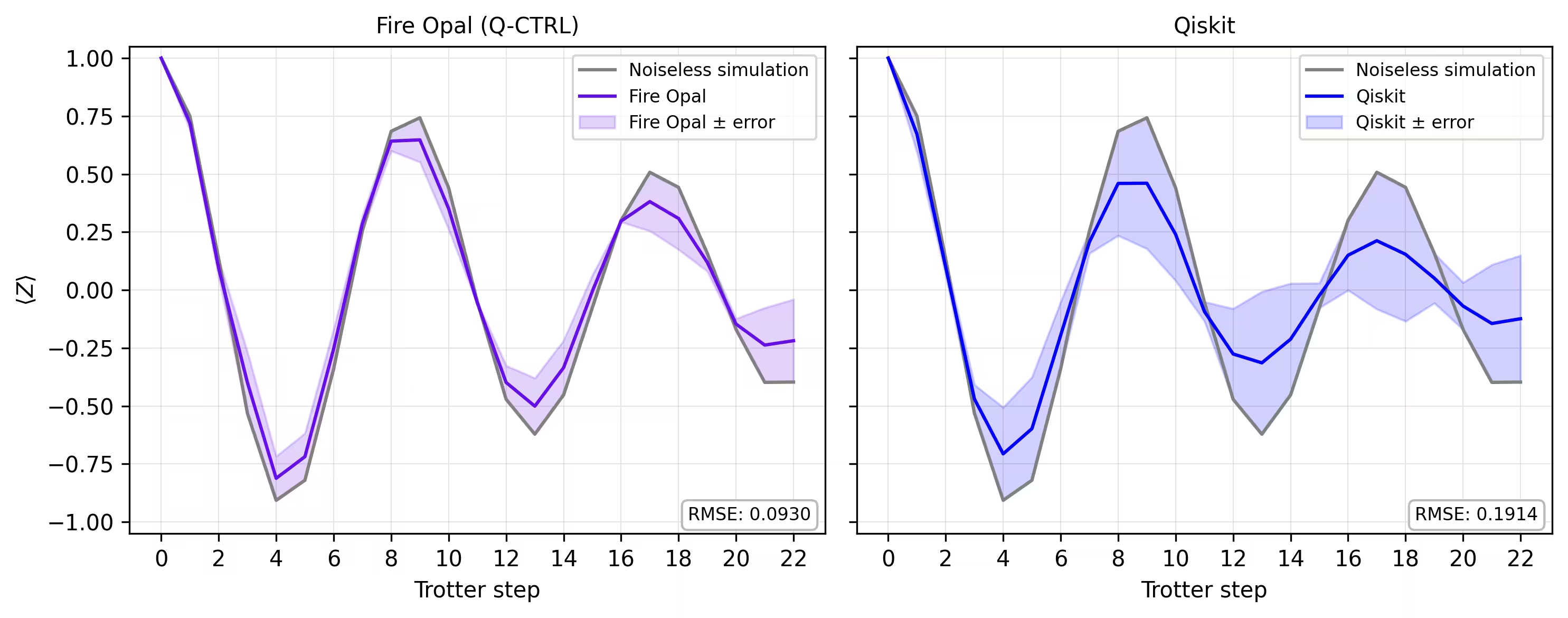
În final, comparăm curba de magnetizare din simulator cu rezultatele obținute pe hardware real. Afișând ambele una lângă alta se poate observa cât de bine se potrivește execuția pe hardware cu Fire Opal cu linia de bază fără zgomot pe parcursul pașilor Trotter.

def make_correlators(test_counts, nq, d_ind_tot):
    mz = np.empty((nq, d_ind_tot))
    for d_ind in range(d_ind_tot):
        counts = test_counts[d_ind]
        for i in range(nq):
            mz[i, d_ind] = z_expectation(counts, i)
    average_z = np.mean(mz, axis=0)
    return np.concatenate((np.array([1]), average_z), axis=0)

sim_exp = make_correlators(sim_counts[0:22], nq=nq, d_ind_tot=22)
qiskit_exp = make_correlators(qiskit_counts[0:22], nq=nq, d_ind_tot=22)

qctrl_exp = [ev.data.evs for ev in result_qctrl[:]]
qctrl_exp_mean = np.concatenate(
    (np.array([1]), np.mean(qctrl_exp, axis=1)), axis=0
)

def make_expectations_plot(
    sim_z,
    depths,
    exp_qctrl=None,
    exp_qctrl_error=None,
    exp_qiskit=None,
    exp_qiskit_error=None,
    plot_from=0,
    plot_upto=23,
):
    import numpy as np
    import matplotlib.pyplot as plt

    depth_ticks = [0, 2, 4, 6, 8, 10, 12, 14, 16, 18, 20, 22]

    d = np.asarray(depths)[plot_from:plot_upto]
    sim = np.asarray(sim_z)[plot_from:plot_upto]

    qk = (
        None
        if exp_qiskit is None
        else np.asarray(exp_qiskit)[plot_from:plot_upto]
    )
    qc = (
        None
        if exp_qctrl is None
        else np.asarray(exp_qctrl)[plot_from:plot_upto]
    )

    qk_err = (
        None
        if exp_qiskit_error is None
        else np.asarray(exp_qiskit_error)[plot_from:plot_upto]
    )
    qc_err = (
        None
        if exp_qctrl_error is None
        else np.asarray(exp_qctrl_error)[plot_from:plot_upto]
    )

    # ---- helper(s) ----
    def rmse(a, b):
        if a is None or b is None:
            return None
        a = np.asarray(a, dtype=float)
        b = np.asarray(b, dtype=float)
        mask = np.isfinite(a) & np.isfinite(b)
        if not np.any(mask):
            return None
        diff = a[mask] - b[mask]
        return float(np.sqrt(np.mean(diff**2)))

    def plot_panel(ax, method_y, method_err, color, label, band_color=None):
        # Noiseless reference
        ax.plot(d, sim, color="grey", label="Noiseless simulation")

        # Method line + band
        if method_y is not None:
            ax.plot(d, method_y, color=color, label=label)
            if method_err is not None:
                lo = np.clip(method_y - method_err, -1.05, 1.05)
                hi = np.clip(method_y + method_err, -1.05, 1.05)
                ax.fill_between(
                    d,
                    lo,
                    hi,
                    alpha=0.18,
                    color=band_color if band_color else color,
                    label=f"{label} ± error",
                )
        else:
            ax.text(
                0.5,
                0.5,
                "No data",
                transform=ax.transAxes,
                ha="center",
                va="center",
                fontsize=10,
                color="0.4",
            )

        # RMSE box (vs sim)
        r = rmse(method_y, sim)
        if r is not None:
            ax.text(
                0.98,
                0.02,
                f"RMSE: {r:.4f}",
                transform=ax.transAxes,
                va="bottom",
                ha="right",
                fontsize=8,
                bbox=dict(
                    boxstyle="round,pad=0.35", fc="white", ec="0.7", alpha=0.9
                ),
            )
        # Axes
        ax.set_xticks(depth_ticks)
        ax.set_ylim(-1.05, 1.05)
        ax.grid(True, which="both", linewidth=0.4, alpha=0.4)
        ax.set_axisbelow(True)
        ax.legend(prop={"size": 8}, loc="best")

    fig, axes = plt.subplots(1, 2, figsize=(10, 4), dpi=300, sharey=True)

    axes[0].set_title("Fire Opal (Q-CTRL)", fontsize=10)
    plot_panel(
        axes[0],
        qc,
        qc_err,
        color="#680CE9",
        label="Fire Opal",
        band_color="#680CE9",
    )
    axes[0].set_xlabel("Trotter step")
    axes[0].set_ylabel(r"$\langle Z \rangle$")
    axes[1].set_title("Qiskit", fontsize=10)
    plot_panel(
        axes[1], qk, qk_err, color="blue", label="Qiskit", band_color="blue"
    )
    axes[1].set_xlabel("Trotter step")

    plt.tight_layout()
    plt.show()

depths = list(range(d_ind_tot + 1))
errors = np.abs(np.array(qctrl_exp_mean) - np.array(sim_exp))

errors_qiskit = np.abs(np.array(qiskit_exp) - np.array(sim_exp))

make_expectations_plot(
    sim_exp,
    depths,
    exp_qctrl=qctrl_exp_mean,
    exp_qctrl_error=errors,
    exp_qiskit=qiskit_exp,
    exp_qiskit_error=errors_qiskit,
)

Referințe

[1] Graph coloring. Wikipedia. Retrieved September 15, 2025, from https://en.wikipedia.org/wiki/Graph_coloring

Sondaj tutorial

Te rog să acorzi un minut pentru a oferi feedback despre acest tutorial. Opiniile tale ne vor ajuta să îmbunătățim conținutul și experiența utilizatorilor.

Link la sondaj

Note: This survey is provided by IBM Quantum and relates to the original English content. To give feedback on doQumentation's website, translations, or code execution, please open a GitHub issue.